Chapter 8: Basic Adjustments Using the Census X11 Method
8.2 Seasonal Adjustment Using Census X11
8.3 Seasonal Adjustment of US E-Commerce
8.4 Seasonal Adjustment of UK Unemployment
8.1 Seasonality
As a motivating example, consider the quarterly series of e-commerce in the US, which was also applied as an example of forecasting in Section 6.5. The series has large seasonal fluctuations: the sales in the fourth quarter are higher than in the first three quarters due to the extra activity among consumers in the period up to Christmas. See Figure 8.1. But the seasonality is not a regular feature because the spike in the fourth quarter in recent years is very pronounced but it was barely visible in the first years of the observation period. It seems impossible to specify the seasonality by an explicit mathematical formula because it varies from year to year.
In this example, seasonality is considered only for monthly and quarterly series. For weekly (and of course also for daily) series, the seasonal structure often turns out to be very unstable, so a reliable seasonal adjustment is impossible. Similarly, variations within a day for hourly observations can be considered as seasonal, but such variations are not the scope for seasonal adjustment procedures. Instead, various trigonometric functions can be fitted to time series with long seasonal periods. That method is described in Chapter 10 with regard to unobserved component models and is exemplified in Chapter 13.
Figure 8.1 Volume of US e-commerce

The purpose of seasonal adjustment is to derive the value of the time series in a situation where no seasonality affects the series. Adjusted values can then be used to compare the real market situation in, say, the third and fourth quarters even if it is evident that sales are always higher in the fourth quarter than in the third quarter due to seasonality. Similarly, specific events in just a single observation can be detected by looking at the adjusted series because the usual seasonal effects are adjusted away.
Seasonality is often due to meteorological conditions such as temperature and rainfall, which affect nearly all human activity. Religious and national days of celebration can also affect a series. These might be fixed dates in the calendar such as Christmas, which affect the series differently according to whether they fall on a Sunday or an ordinary working day. Some religious festivals occur in a very unsystematic way, such as Christian Easter and Muslim Ramadan, both of which are timed by the phases of the moon and thus vary from the Gregorian calendar. For specific time series, other seasonal variations exist. Think of the sales of flowers for Mother’s Day (the date of which varies according to local traditions from country to country). In the seasonal adjusted series, the effects of all such events should be extracted, leaving only the effects of level and the specific events in the adjusted value.
Of course, the existence of a seasonal adjusted series is very hypothetical because the adjusted series cannot be observed and often the existence of such series is hard to believe in. It is somehow unrealistic to think about the sale of toys in December in a world where the Christmas season had not been invented. However, the seasonal adjustment procedures as presented here seem rather intuitive, and they are broadly accepted.
Seasonal adjusted values are regularly published by national statistical offices and great interest is attached to them. The figures for unemployment, price indices, and so on, have great impact on stock exchanges and on the political process. It is therefore important that the underlying calculations are valid and trusted. They must in no way be affected by subjective manual corrections.
Many official statistical bureaus apply the so-called X11 method. This method has been developed over a long span of years by the US Census Bureau from version 1 in 1954 to X11 in 1965. See, for example, Ladiray and Quenneville (2001). The method is implemented by many software providers and is available for free from the U.S. Bureau of the Census (2001). In SAS, it was first implemented as PROC X11, and many refinements were later added in PROC X12. These extensions include the X11-ARIMA method as developed by Statistics Canada. See Dagum (1988). Even if these methods are rather old, they are by no means obsolete. The X11 method still forms the basis of most seasonal adjustments.
8.2 Seasonal Adjustment Using Census X11
The original series Xt is considered as a sum of three components
Xt = TCt + St + It.
The component TCt denotes a trend cyclic component, which corresponds to the level of the series. This name reflects that this component is meant to include both trends and business cycles. This is necessary because many time series include trends. For example, many series in economics and business have trends due to inflation and economic growth, and phenomena such as aging in biological processes can also be considered as a trend.
The notion of cycles in this connection is somehow confusing. The word cycles has nothing to do with seasonal behavior even if the seasonal variation throughout a year in many practical series looks like a sinusoid cycle. Most meteorological measurements such as monthly temperatures look graphically like deterministic waves. The term cycles originates from the theory of economic cycles in economic history where some cycling behavior is often seen for yearly series. Cycles are also observed in other sciences, the nearly 11-year period in sunspot activity being a famous example.
In the context of seasonal adjustment, there is, however, no need to distinguish between the trend and the cyclic component. (See Chapter 10 on unobserved component models for a further treatment of specific underlying components of an observed time series.) The trend cyclical component, TCt in the seasonal adjustment setup is just considered as the actual level of the observation in the hypothetical situation that no seasonality exists and that nothing unusual happens.
The irregular component It is the remainder term that includes everything that refers only to the present observation for the actual month of the series in the actual year. It can be considered as the unusual part of the observation. It is not a part of the actual level of the series and cannot be explained by the seasonal behavior.
The seasonal component St can be seen as a component that represents a given effect during the same month of each year in the series. The subscript t in this notation mainly reflects the month, meaning that St should have only twelve values for monthly observations and should attain the same value (for example, the month of May) each year. However, the seasonal structure of time series in practice is never completely constant, and the seasonal component necessarily has to be somewhat time varying. A global example is the monthly price of apples, which obviously is affected by the seasonality in the harvests but increasing trade between the northern and the southern hemisphere tends to diminish this seasonality. So even if the sub index t in the notation St for a seasonal component reflects only the calendar month of the observation, the value of St is not exactly equal to St-12 but is allowed to differ a bit.
As the trend-cyclic component is meant to represent the level of the series, the components St and It on average should be 0 in this additive formulation. A positive value of St then solely corresponds to a month of the year with values above the overall level. Similarly, a negative value of It corresponds to a month in which the observed value of the series is for some reason below the expected value, given both the level and the seasonal effect.
The trend-cyclic component TCt for a particular month t can be estimated by simply averaging the series for, say, 12 months before and after the month t, Xu u = t - 12 ,...., t + 12. However, special weights should be used in order to balance the average. In the case where t corresponds to the month of May, three observations for the month of May are included in the average, but all other months are included only twice. The average is then defined as:
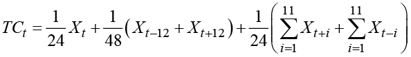
The calculation of the trend-cyclic component TCt is in practice not just performed by simply averaging neighbor values using equal weights. Instead, weighted averages are used because the theory of smoothing of series leads to weights that result in desirable properties, especially regarding the smoothness (“differentiability”) of the resulting trend-cyclic component, TCt. This type of moving averaging turns the series Xt into a smooth curve by formulas of the basic form

where all the weights ωi sum to 1. The weights ωi are usually derived by Henderson’s formula (see, for example, Ladiray and Quenneville [2001]), but their precise definition is of no practical interest for the user. For mathematical reasons, the weights ωi are not necessarily nonnegative, in order to obtain a smooth estimated trend curve. In practice, the number of terms k = 2m +1 is chosen as some odd number, often 9 for quarterly data and 13 or 23 for monthly series. The more terms included in the moving average, the smoother the estimated trend curve appears. This is discussed in Section 9.3.
In the beginning and the end of an observed time series, the above symmetric averaging is of course impossible. This problem is of great concern because the most recent value is often the most important. For this last observation, only the observations for past years are known but all the future observations are, of course, unknown. This problem is theoretically circumvented by applying special weights in the outmost parts of the series. Another possibility is to forecast the series so that symmetric averages can be calculated using forecast future values. This possibility is included in the seasonal adjustment procedures; see Section 9.1. If the forecasts are reliable, this procedure is promising. One consequence is that the seasonally adjusted values change as more recent observations become available. This is, however, inevitable, and institutions often form a policy for such revisions in their publishing policy.
The seasonal component for the month of May, for example, can be estimated as the average of Xt - TCt for all t’s that correspond to the months of May. This average is calculated using appropriate weights by the lines argued previously in order to obtain theoretically reasonable values. Often the calculations are performed by averages of the form

using an interval of two years before and two years after the actual month. The weights intuitively should give more emphasis to the actual observation. For the outmost observations, especially the most recent observation, the weights have to be adjusted or forecast values have to be applied. It is important to note that the seasonal component St is calculated in a flexible form so that the estimated values of St are non-constant, corresponding to a time-varying seasonal structure. On the other hand, averaging over five years leads to an estimated seasonal component that is somewhat robust to irregularities in the actual observation. You can achieve this by changing the length of the interval in the averaging formula.
The irregular component is then at last calculated as the remainder term Xt - TCt - St, using the above estimates for TCt and St. If the components TCt and St are calculated properly, this definition of the irregular component reflects all variation in the series that affect only this particular observation. Most actual series have various outliers. For example, a series of production figures might drop dramatically one particular month because of a labor market conflict. This drop is, in the strict decomposition previously described, considered to be a part of the irregular component. But the exceptional low value leads to very low values of the derived trend-cyclic component because it will affect the moving average for all months close to the outlier even if intuitively the level should be unaffected.
Such outliers are detected in the algorithms by automatic procedures, and their effects are then compensated for. This is done iteratively so that outliers defined as extreme differences between Xt and preliminary calculations of TCt and St are removed, giving rise to new calculations of TCt and St, and so on. Outliers are detected as extreme values of the irregular component compared with a standard deviation that is locally estimated using only values of the irregular component a few years before and after each observation. A value less than 1.5 times the standard deviation in absolute terms is not at all considered an outlier, and values larger than 2.5 times the standard deviation in absolute terms are identified as outliers. Values between 1.5 and 2.5 times the standard deviation are considered partial outliers. The trend-cyclic component and the seasonal component for these outliers are then calculated using a modified value of the observation. This modified observation is calculated as an average of neighboring observations, giving the actual observation weight zero for clear outliers and reduced weight for partial outliers.
In the X11 algorithm, these modifications are done in many iterations in order to obtain a robust end result that works properly for all types of seasonal time series met in practice. This careful correction for outliers is a major feature of the X11 method. The actual algorithm is based on the experience of the many years previous to the X11 version. For the user, all this is of no practical interest and the details are hidden in rather non-informative tables in the output. Ladiray and Quenneville (2001) present a rigorous documentation of the algorithm.
In practice, the formula for the decomposition in three components is more often formulated as a multiplicative expression instead of using addition. This results in the formulation
Xt = TCt × St × It .
In this way, the seasonal effect of a particular month is interpreted as a relative effect (for example, a 10% increase, and not an absolute effect, such as extra sales of $1 million). This can be achieved simply by using a logarithmic transformation, or the calculations can be described by multiplication and division instead of addition and subtractions. Of course, other transformations can be applied as well in order to stabilize the original series Xt. This discussion is parallel to the discussion of appropriate forecasting models in Section 6.4. In short, the additive variant is best in series with a fairly constant level, and multiplicative versions prove better for series with a trending behavior.
In practice, you often want the adjusted series of, say, a monthly time series to add up to the actual observed annual total. Similarly, the seasonal component in the additive version intuitively should sum to 0, and in the multiplicative version the seasonal factors should on average be one. All the iterative manipulations of the data series do not guarantee, however, that this is automatically the case. Often this is obtained by a final modification of the estimated components and adjusted values by multiplication with correcting factors.
8.3 Seasonal Adjustment of US E-Commerce
The code in Program 8.1 is the minimal code necessary to perform a seasonal adjustment of the series of quarterly e-commerce, which was also considered in Section 6.5. The assignment of the variable date as a date variable formatted by SAS automatically tells the program that data consists of quarterly observations.
Program 8.1 A simple code for seasonal adjustment
PROC X12 data=sasts.Ecommerce date=date;
var Ecommerce;
x11;
run;
This standard setup of the PROC X12 procedure performs a seasonal adjustment using the original X11 algorithm by using the X11 statement. An alternative that provides identical results is to apply PROC X11. The seasonal adjustment is by default based on a multiplicative decomposition with no further refinements. Various intermediate series with details of the modifications for outliers during the iterative calculations of TCt, St, and It are printed to the output window. See the SAS documentation and Ladiray and Quenneville (2001) for details about the definition of these series.
Some of the series are also by default plotted as poor-quality line plots in the output. The procedure does not provide high-quality plots of the series in the decomposition of the original series in a seasonal adjustment. The ODS Graphics System offers only plots of autocorrelation, spectra, and some forecasts, which are also generated by PROC X12.
In order to plot the most interesting series, you have to store them in new data sets by using an OUTPUT statement, as shown in Program 8.2.
Program 8.2 A simple code for seasonal adjustment with series output stored in a new data set
PROC X12 data=sasts.Ecommerce date=date;
var Ecommerce;
x11;
output out=out a1 d10 d11 d12 d13;
run;
Here the output statement stores the most relevant series in the new data set Out. The output series are named following the original X11 notation:
a1: the original time series Xt
d10: the seasonal component St
d11: the adjusted series, defined as TCt + It
d12: the trend-cyclic component TCt
d13: the irregular component It
In order to identify the outputted series, the naming convention is that these abbreviations are prefixed by the variable name of the original series. In this situation, where the original series is given as the variable Ecommerce, the adjusted series is named Ecommerce_d11. In the output data set, the variables are labeled according to the X11 notation so that the variable Ecommerce_d11 is labeled “Table D11: Final Seasonal Adjusted Data.” These series are all plotted using a sequence of applications of PROC SGPLOT with the code in Program 8.3.
Program 8.3 Plotting the components from the X12 decomposition by PROC SGPLOT
PROC SGPLOT data=out;
series x=date y=Ecommerce_A1/markers;
series x=date y=Ecommerce_D11/markers;
xaxis values=(‘1jan99’d to ‘1jan11’d by year);
run;

PROC SGPLOT data=out;
series x=date y=Ecommerce_D10/markers;
xaxis values=(‘1jan99’d to ‘1jan11’d by year);
run;
PROC SGPLOT data=out;
series x=date y=Ecommerce_D12/markers;
xaxis values=(‘1jan99’d to ‘1jan11’d by year);
run;

PROC SGPLOT data=out;
series x=date y=Ecommerce_D13/markers;
xaxis values=(‘1jan99’d to ‘1jan11’d by year);
run;
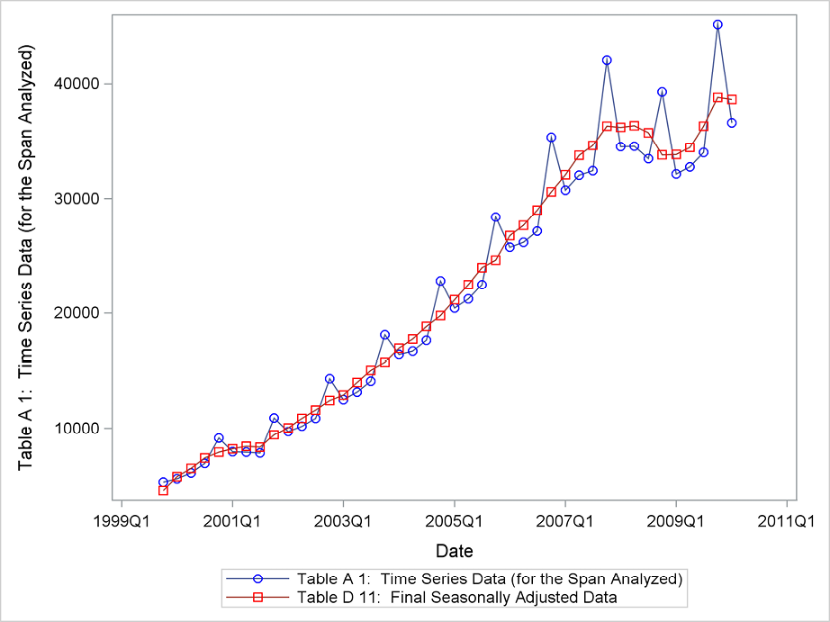
Figure 8.2 is a comparison between the original series and the final seasonal adjusted series, plotted in the same plot. This plot clearly proves that the seasonal adjustment has done the job because none of the original seasonality is left in the adjusted series.
Figure 8.2 Original series of Ecommerce compared to the seasonal adjusted series
The trend-cyclic component is dominated by a steep upward trend with a sudden decline due to the financial crises beginning in the third quarter of 2008, but after just a few quarters the trend is back again. See Figure 8.3.
Figure 8.3 Trend-cyclic component for US e-commerce

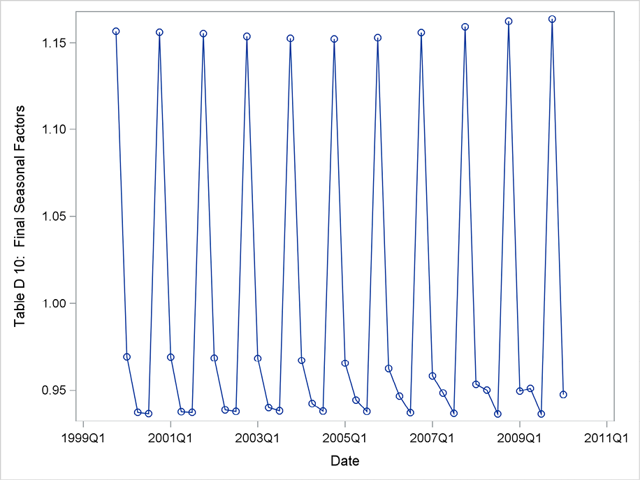
The seasonal component mainly reflects that the series attain high values in fourth quarters. (See Figure 8.4.) In this multiplicative version of the adjustment procedure, values around 1.15 of the seasonal factor correspond to a 15% increase of the value of e-commerce, due to the Christmas season. Another observation from Figure 8.4 is that the seasonal factor for the first quarter is declining over the observation period. This could be due to the definition of the series because payments for e-commerce are registered more quickly as this type of business expands.
Figure 8.4 Seasonal component for US e-commerce
The irregular component, which is plotted in Figure 8.5, presents some marked events. The low value 0.96 in third quarter 2001 is the most remarkable value, which corresponds to a 4% lower value of e-commerce than what was expected.
Figure 8.5 Irregular component for US e-commerce

This series is revisited in Section 9.2, where more advanced analyses than simple seasonal adjustments included in PROC X12 are applied. Moreover, the possibilities for extracting unobserved components using PROC UCM are applied to the series of e-commerce in Chapter 12.
8.4 Seasonal Adjustment of UK Unemployment
In this section, the time series of the monthly numbers of unemployed in the UK for the period January 1955 to February 2011 is seasonally adjusted, using only the simplest original techniques offered by X11. The main point of this example is to demonstrate the flexibility and generality of the method. The series is very long with many shifting levels, including shifts in the seasonal component.
The series is pictured in Figure 8.6 for the entire span of years. This monthly time series hardly shows a seasonal pattern, unlike the more detailed plot of the data for just a few years, even if high values in the winter months are expected due to higher unemployment caused by the weather. (See Figure 8.7.) A plausible explanation for the seemingly non-seasonal behavior might be that the underlying changes in the level of unemployment due to the shifting economic conditions dominate the seasonal component. The adjustment procedure in this section, however, gives another picture. The seasonal component clearly has a huge impact.
Figure 8.6 UK unemployment
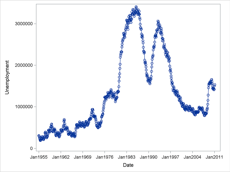
Figure 8.7 Monthly data UK unemployment for four years

Program 8.4 uses PROC X12 to obtain a seasonal adjustment through the original X11 method using the default multiplicative version.
Program 8.4 Seasonal adjustment of the monthly UK Unemployment series
PROC X12 data=sasts.UK_unemployment date=date;
var unemployment;
x11;
output out=out a1 c17 d10 d11 d12 d13;
run;
The most important series are stored in an output data set for later use by the OUTPUT statement. The seasonal factor is plotted in Figure 8.8. The seasonal behavior of the unemployment series has changed over the years. In the 1950s, the effect of seasonality was very pronounced, with about a 20% higher level in the winter months and 20% lower values in the summer months compared with the estimated adjusted level of the unemployment. But the seasonal fluctuations are reduced to approximately +/- 5% from around 1980.
Figure 8.8 Seasonal component for UK unemployment

In the irregular component, some outliers of an order of about +/- 5% are present. (See Figure 8.9.) The effect of these outliers is compensated for in the seasonal adjustment algorithm, as described in Section 8.2. In the printed output, the treatment of possible outliers is documented by many series. These series are usually only of minor interest. Refer to the SAS documentation for details and to Ladiray and Quenneville (2001) for a more theoretical description.
An example of the series, the C17 series, is written by the OUTPUT statement and then plotted in Figure 8.10. This variable is defined as the weights to the actual calculated value of the irregular component, expressed as a percentage. The value 100% corresponds to observations having full weight in all calculations. Observations that are totally disregarded have the value 0%. Many observations are given weights between 0% and 100%, indicating that they are only partly included in the calculations; the other part is defined by smoothed values of neighboring observations. In most practical situations, this series gives enough information to identify outliers of the series for further study, and rigorous outlier testing is unnecessary.
Figure 8.9 Irregular component for UK unemployment

Figure 8.10 Corrections for outliers in the adjustment procedure

The main lesson from this example is that the seasonal adjustment procedure is adapting to new structures over this long span of years. In traditional statistical analysis, a model of this time series would in some sense be considered static, which is obviously erroneous in light of the shifting economic climate. Correction for trading days is, for example, impossible because it is hard to believe that estimated regression coefficients could be constant over this span of 55 years. But the X11 algorithm includes an intelligent “forgetting” algorithm. Therefore, whether the observation period begins fifty years ago or just a few years ago is unimportant for the adjustment of recent observations.