Chapter 4: Interpolation Using PROC EXPAND

4.1 Interpolation of Time Series

4.2 PROC EXPAND

4.1 Interpolation of Time Series

Most SAS procedures require that the time series be observations equidistant in time. This means that a problem appears if one observation is missing, such as when no information is available for a month. For a series of total sales of a particular item, no sales information within a month in principle means no sales at all that month. But such missing observations could be due to errors in the accounting systems. If so, no registrations does not mean a zero value. The price of a share at a stock market is typically recorded every time the share is traded, but in theory, it could also be traded at other points in time and not recorded. The price is not zero just because there was no trade. Similar examples appear in medicine, where measurements of, say, blood sugar level could be missing due to some type of error in the measurement equipment.

It is possible to interpolate data series in order to find reasonable values for the missing observations. Interpolation is ideally performed by the inclusion of knowledge of the actual content of the time series. Alternatively, simple manual interpolations can be performed in the SAS DATA step. More formally, however, SAS offers a procedure for interpolation, PROC EXPAND, described in the next section.

4.2 PROC EXPAND

PROC EXPAND interpolates missing observations in time series by simple curve-fitting methods. One simple possibility is to join the points in a diagram of the available observed values by straight lines, and then find the missing values on these connecting lines. You can easily develop this idea by fitting a smooth curve through the available points by spline-curve fitting, and then again simply recording the values that are missing from this fitted curve.

In this section, the example of the copy machine from Section 3.2 is continued. The problem is that the number of copies made during a period in time is observed only at very irregular intervals of a few days to several months. This means that aggregation by PROC TIMESERIES, as described in Section 3.2, cannot provide reasonable numbers for months when no observations exist. But an application of PROC EXPAND will do the job through its facilities for interpolation.

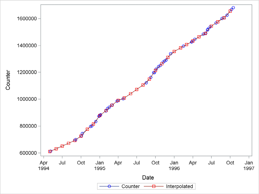
Program 4.1 shows an application of PROC EXPAND that interpolates the series of readings of the counter on the machine by straight lines. The counter position is interpolated linearly in the interval between the actual observations, as illustrated in Figure 4.1. The method is simply to read the values from the curve where the actual observations are connected by straight lines as stated by method=join in the CONVERT statement. The interpolation of the counter position is performed to the aggregation level of months by the to=month option in the procedure call. The time index is a necessary input to the procedure in the ID statement where the variable has to be in SAS datetime format. In the CONVERT statement, a new name for the interpolated values of the counter series is given as the variable name after the equality sign. The original series and the interpolated series are finally merged in the DATA step in order to plot the result by PROC SGPLOT.

Program 4.1 A first application of PROC EXPAND

PROC EXPAND data=sasts.copy_machine out=joinB to=month;
convert counter=interpolated /  method=join;
id date;
run;
data d;
merge sasts.copy_machine joinB;
by date;
run;
proc SGPLOT data=d;
series x=date y=counter/markers;
series x=date y=interpolated/markers;
run;

Figure 4.1 Interpolated counter positions

For this example, the most relevant result is the series of first differences of the output series because it represents the interpolated series of copies made each month. In Program 4.2, these differences are calculated by the function dif in a separate DATA step and then plotted by PROC SGPLOT.

Program 4.2 Calculating the number of copies using the interpolated series of Program 4.1

data e;
set joinb;
number=dif(interpolated);
run;
PROC SGPLOT data=joinb;
series x=date y=number/markers;
run;

Figure 4.2 Number of copies interpolated to a monthly frequency

PROC EXPAND offers lots of facilities for the transformation of the input (the original) series and the output (the interpolated) series. In fact, the differences that were created in a separate DATA step in Program 4.2 could be generated by PROC EXPAND as a transformation of the output series by the option transformout=(dif 1). See Program 4.3. This provides exactly the same output series result.

Program 4.3 An example of the transformation facilities in PROC EXPAND

PROC expand data=sasts.copy_machine out=joinB to=month;
convert counter=number /  transformout=(dif 1) method=join;
id date;
run;

PROC EXPAND also includes features for estimating unobserved components such as extraction of trends and seasonalities. However, because SAS provides a special procedure for such analyses, PROC UCM (unobserved component models), which includes more facilities, PROC UCM is used in Part 5. See the SAS documentation for information about further analyses offered by PROC EXPAND.