Chapter 11: Analysis of Danish Fertility Using PROC UCM
11.1 Component Estimation
In this section, PROC UCM is applied in an analysis of the series of Danish fertility for the years 1901 to 2009. This series was also considered in Chapter 5 and Chapter 7 as an example of exponential smoothing and other forecasting methods.
Most of the code lines in the application of PROC UCM in Program 11.1 are specifications of plots and output components. In the ID statement, the time identification variable (in this example, the variable year) is specified. The time series for this particular example is specified as yearly observations by the option interval=year. The name of the time series to be decomposed is, as in many other SAS procedures, specified in a MODEL statement. The OUTLIER statement is discussed in the next section.
Program 11.1 The basic model in PROC UCM
ods graphics;
PROC UCM data=sasts.Fertility;
id year interval=year;
model fertility;
level plot=(filter smooth);
outlier;
estimate plot=all;
forecast lead=24 plot=forecasts alpha=0.1;
run;
ods graphics off;
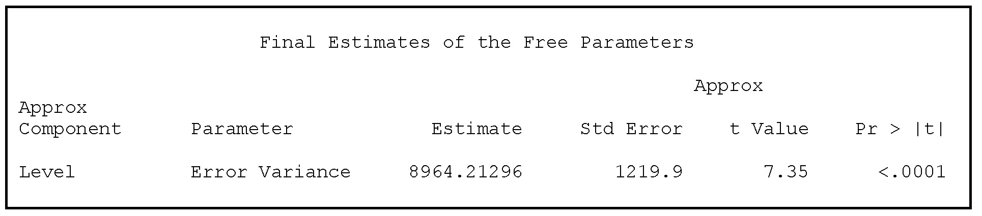
The estimated variance for the noise series in the level component is printed in the output window; see Output 11.1. The variance of the estimated innovation term in the level component, 8964, is large. It is in fact larger than the variance of the yearly changes in fertility, which is 8591, as you can see by an application of PROC UNIVARIATE. A more relevant comparison is perhaps the uncorrected sum of squares (divided by the number of observations) for the yearly differences, which also equals 8964 and which you can also see in output provided by PROC UNIVARIATE. The practical impact is that the fitted-level component equals the observed series with almost zero residuals.
Output 11.1 The estimated component variance
For the level component, both the filtered and the smoothed plot are drawn by the option plot=(filter smooth)in the LEVEL statement in Program 11.1. The filtered plot, Figure 11.1, is defined using only past observations, so that only observations previous to but not later than time t are included in the calculation of the level at time t. In the smoothed version, Figure 11.2, all observed values both before and after time t are used in the calculation of the level at time t, leading to a smoother ex post plot. The plots look very similar, but because the smoothed plot is based on more observations, the confidence limits in the observation period are narrower.
The forecasts are defined using the latest observed value of the level. The forecasts form a constant horizontal line because no trend is incorporated in the model so far. The confidence limits are broad for longer horizons, even when the confidence level is specified at α = 10% by the option alpha=0.1 in the FORECAST statement instead of the more commonly used default value α = 5%. Note that the confidence limits for forecasts in the filtered and the smoothed plots are identical in the forecasting period. This is the case because the forecasts are based on all available observations in the observation period.
Figure 11.1 The level component for the fertility series estimated by the filtering algorithm

Figure 11.2 The level component estimated by the smoothing algorithm

11.2 Outlier Detection
The residuals are plotted in Figure 11.3. This plot (among others) is requested by the plot=all option in the ESTIMATE statement. The most dominant residuals are for the years 1919 and 1920, but a positive residual in 1941 and the negative residuals in the late 1960s also seem significant. The OUTLIER statement produces a formal outlier test, shown in Output 11.2. In this test, a dummy component for each year is applied for each observation, and if this component is tested as significant, the observation is printed as an additive outlier. These tests exclude the influence of potential outliers on both the residual and the level component, so the results are not a simple replication of what is shown in the residual plot. The estimates for the printed outliers are estimated for the dummy component, which is intended to compensate for the outlier. The sign of the estimate in Output 11.2 is for that reason the opposite of the sign of the corresponding residual in Figure 11.3. As noted in Section 5.13, the outliers for the years 1919–1920 are probably due to registration errors during the years of the Danish reunification with the southern parts of Jutland.
Figure 11.3 Residuals for the fitted level model for the fertility series

Output 11.2 Outliers

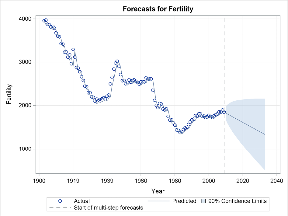
Figure 11.4 Fit and forecasts from the basic model to the fertility series

As previously noted, the largest forecast errors are found for the years 1919, but the fit for the remaining years seems good. A closer look reveals, however, that the forecasts in the forecast plot (Figure 11.4) seem to mirror the observations always one year behind! We saw this also in the forecasts in described in Section 5.3.
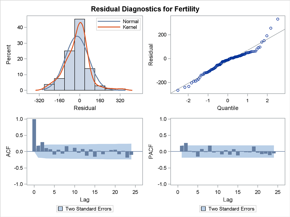
The plot=all option in the ESTIMATE statement also produces a panel plot, Figure 11.5. This panel contains a histogram and a Gaussian probability plot for the residuals that show that the hypothesis of normally distributed errors seems acceptable. The autocorrelation plot that is also included in the panel in Figure 11.5 points at some positive autocorrelations for lags one to five. This means that the model is capturing a new level of fertility only after some years’ delay. The first two partial autocorrelations are positive, which indicates that an autoregressive model might be suitable. In the last part of this chapter, we will return to this problem of autocorrelation by including a second-order autoregressive model, AR(2), for the residuals.
Figure 11.5 Panel plot for fit of the basic model
In the text output, the level component is printed as requested by the print option in the LEVEL statement. You could save the level component using the ODS table for use as input in models for other series. The forecasts are printed by default.
11.3 Extensions of the Model
The model can be extended with a slope component in order to specify the trend model described in Section 10.3. To do so, include a SLOPE statement, as in Program 11.2. The option plot=smooth in both the SLOPE and LEVEL statements of Program 11.2 specifies that only the smoothed version of the level and the slope components are plotted.
Program 11.2 Including a trend component
ods graphics;
PROC UCM data = sasts.Fertility;
id year interval = year;
model fertility;
level plot=smooth;
slope plot=smooth;
outlier;
estimate plot=all;
forecast lead=24 plot=forecasts alpha=0.1;
run;
ods graphics off;
The slope component, shown in Figure 11.6, varies according to the local trending behavior in the observed series. The slope component shows fertility declining for approximately the first 30 years, but shows fertility as being rather constant for about 50 years, although with large fluctuations. The slope component is significantly negative for the first 30 years during which fertility declines at a stable rate, but since 1930, the slope component is more volatile. From an overall perspective, it could be considered zero because a trend intuitively cannot change so rapidly.
Figure 11.6 The slope component estimated by the smoothing algorithm

Output 11.3 Estimates for the level and trend variances

The estimated variances, Output 11.3, show that the variance for the slope is insignificant. In spite of the discussion above, the slope can be considered as a constant instead of as a time-varying component. The slope is fixed by fixing the variance to 0 in the slope statement. The option var=0 gives the value 0 as an initial value for the variance parameter. The option noest specifies that this parameter is not estimated along with the other model parameters.
slope plot=smooth var=0 noest;
In this situation, the slope parameter is a constant. This constant slope parameter is significant as reported in the table of states of the level and slope component for the last observation in Output 11.4. The estimated coefficient - 21.3 is numerically larger than twice its standard error. Fertility is accordingly modeled as having a fixed negative trend. This could, of course, be seen as an acceptable rough fit to the observed fertility for the more than 100 years in the sample period. But when it comes to forecasting, it seems unrealistic when you see the forecast plot, Figure 11.7. Steady, linearly decreasing fertility means that the Danish population will soon die out. The time-varying slope component in the original code of Program 11.2, which is plotted in Figure 11.6, ends up as almost zero for the latest observations. This corresponds to an almost horizontal trend in the forecasting period, which is more reasonable, even if the variance parameter is only insignificantly positive.
Output 11.4 Estimated level and trend for the last observation

Figure 11.7 Forecasts of Danish fertility in a model with a constant trend
As an alternative to a slope component, you could incorporate a cycle component into the model. This component has the form of a sinusoid, which can be defended by some demographic considerations. In the code, it is easily done by including a CYCLE statement, as in Program 11.3.
Program 11.3 Including a cycle component in PROC UCM
ods graphics;
PROC UCM data = sasts.Fertility;
id year interval = year;
model fertility;
level plot=smooth;
cycle plot=smooth;
outlier;
estimate plot=all;
forecast lead=100 plot=forecasts alpha=0.1;
run;
ods graphics off;
This results in a cycle with a wavelength at 53.6 years, which is too long to provide a clear demographic interpretation. (See Output 11.5.) The wavelength can be used as an approximation of the trending behavior of the series for the first 50 years. The damping factor is estimated to be 1, which is clearly a sinusoid curve in the forecast plot, Figure 11.8. The plot extends the forecast period to 100 years in order to make the forecasting properties more visible.
Output 11.5 Estimates of cycle period and level variances

Figure 11.8 Forecasts of the fertility series using a cycle model

As noted in the first part of this chapter, some autocorrelation problems exist in the model with the level as the only component. The autocorrelations are also present in the model with the cycle component and in the fixed-trend slope model. But the autocorrelation problems disappear in the more flexible model with the time-varying slope. Autocorrelations can be introduced to the models in many ways by PROC UCM, examples of which are illustrated in the other chapters about unobserved component models. In this analysis, the lagged fertility variable, which is the dependent variable in the model, is included by the DEPLAG statement. This statement includes just one lag, as specified by the option lag=1. See Program 11.4.
Program 11.4 Including lags in PROC UCM
ods graphics;
PROC UCM data = sasts.Fertility;
id year interval = year;
model fertility;
deplag lag=1;
level plot=smooth;
outlier;
estimate plot=all;
forecast lead=100 plot=forecasts alpha=0.1;
run;
ods graphics off;
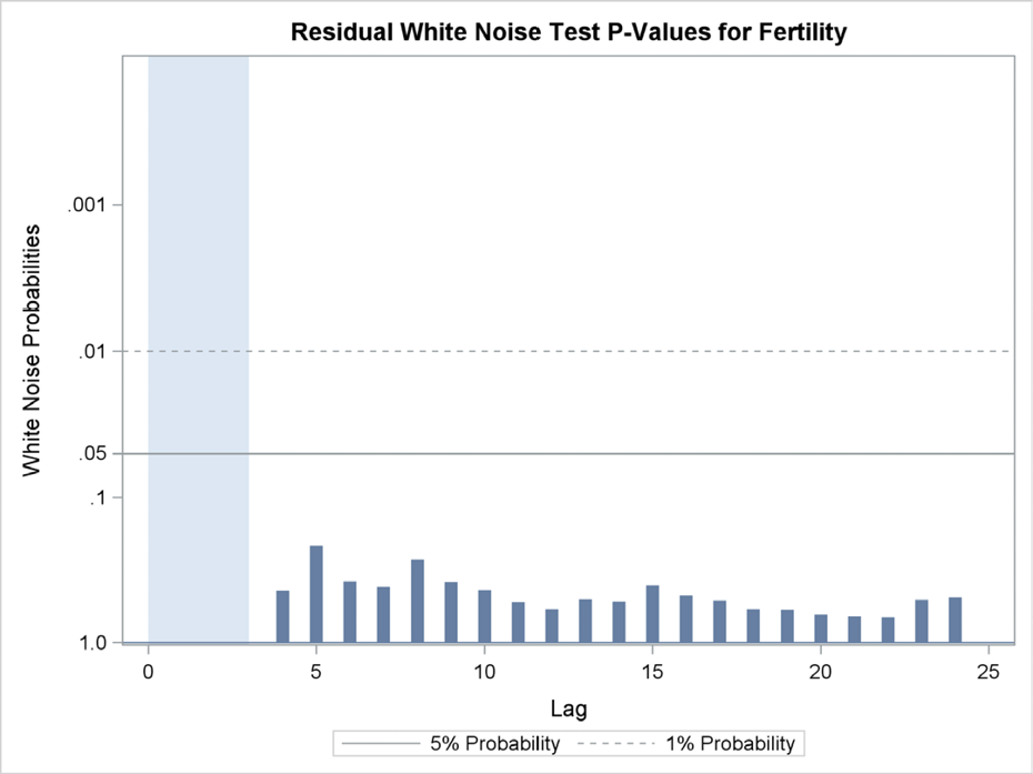
In the estimate statement for the application in Program 11.4, all available plots are specified by the plot=all option. Among these plots is a more detailed picture of autocorrelation tests with a plot of the p-values at a logarithmic scale with clear indications of the most significant interesting levels for testing. You can clearly see in Figure 11.9 that the p-value for these tests for all lags are at the 1% limit or lower, meaning that the autocorrelation problem is still not solved by just one lag of the dependent variable.
Figure 11.9 Testing p-values at a logarithmic scale for autocorrelation testing

The autocorrelation problem for this data series could be solved by including two lags instead of just one of the dependent variable, which is provided by the following statement:
deplag lag=2;
The lag=1 parameter is insignificant, but the lag=2 parameter is clearly significant; see Output 11.6. The white noise test of no autocorrelation shows p-values clearly above 10%, and the model fit is accepted. (See Figure 11.10.) The resulting model is, however, more descriptive than interpretable because the strict interpretation of the lag=2 parameter is that Danish women give birth every second year. The forecasts are by no means superior to the forecasts calculated in Section 5.3 by PROC ESM, which is a simpler forecasting procedure.
Output 11.6 Estimated lag parameters and level component variance
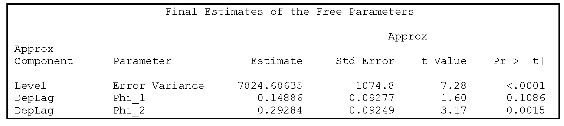
Figure 11.10 Autocorrelation tests for residuals of the model that includes two lags