
Chapter 12: Analysis of US E-Commerce Using PROC UCM
12.1 Estimation of the Components
12.1 Estimation of the Components
In this chapter, PROC UCM is applied in an analysis of the series of e-commerce, which was also considered in Section 6.5. This application of PROC UCM is intended to demonstrate some of the more advanced modeling abilities of the procedure, including the use of independent variables. However, in the first application shown in Program 12.1, only a simple level-trend model (also used in Chapter 11) is used in combination with a seasonal component. The three components are specified by the LEVEL, SLOPE, and SEASON statements. In the SEASON statement, the seasonal length is specified as 4 because the series is quarterly. The plotting options are set so that only the smoothed component estimates are plotted.
Program 12.1 Decomposition by PROC UCM into a level, a trend, and a seasonal component
ods graphics;
PROC UCM data=sasts.E_commerce;
id date interval=quarter;
model E_commerce;
level plot=smooth checkbreak;
slope plot=smooth;
season length=4 plot=(smooth s_annual);
outlier ;
estimate plot=(panel);
forecast lead=24 plot=forecasts alpha=0.1;
run;
ods graphics off;
In Figure 12.1, the results seem somehow disappointing. The slope component is rapidly changing during the financial crises of 2007−2010 as the slope changes from being significantly positive to significantly negative during two quarters. This outcome can be explained as the effect of the crises by looking at the estimated level series, shown in Figure 12.2. As with the fertility example in Chapter 11, this result is not what is naturally expected. A trend intuitively has to be persistent, and even if it could change over time, only small variations would be allowed. In other words, the estimated variance of the slope component is too high. This problem can be remedied by specifying a lower value for the variance of the slope component.
Figure 12.1 Slope component estimated by Program 12.1

Figure 12.2 Estimated level component using Program 12.1

Output 12.1 Estimated component variances and fit statistics
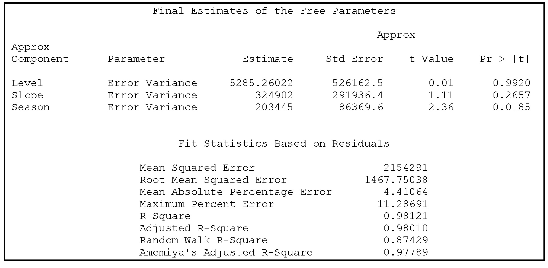
The estimated parameters and some diagnostics for model fit are given in Output 12.1. The variances of the slope and level components are both insignificant. The fit is almost perfect with R2 = 0.98. This gives a clear indication that the model is over parameterized, leading to a too-perfect fit for which the model tells nothing more than the observed series alone. One possibility is to fix one of the variances in the numerical estimation algorithm. In the statement below, the slope is fixed at a constant value because the innovation variance for the slope process is fixed at 0. In this way, a model with a linear trend that is fixed, although at varying intercepts, is included for the volume of e-commerce.
slope plot=smooth var=0 noest;
This might be a reasonable possibility for these data, but it also possible that a specification of a positive variance, but that is one less than the estimated value in Output 12.1, would perform even better. A variance of 10000 is specified by:
slope plot=smooth var=10000 noest;
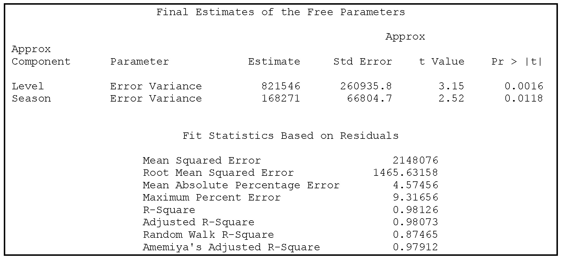
For this specification, the parameter estimates seem reasonable and the fit is not much worse; see Output 12.2. The slope component varies only a very little, and the trend for that reason is much more stable; see Figure 12.3. The level plot, Figure 12.4, more precisely mimics what intuitively could be the underlying tendency of the growth in e-commerce, with a clearer U-shape around 2009. Moreover, the confidence interval in the forecasting period is much smaller than in Figure 12.2, when an estimated trend was incorporated in the model.
Figure 12.3 Slope component estimated with a small fixed variance

Figure 12.4 Estimated level component using a small slope component variance

Output 12.2 Level and seasonal component variance in a model with fixed slope component variance
If the slope component is fixed by the options var=0 and noest, the slope is constant and the estimated value, 850, is printed as the estimated value for the last observation in the table in Output 12.3. The conclusion is that the value of e-commerce increases steadily by 850 million dollars each quarter, adjusted for seasonal variation. This trend is partly due to inflation and economic growth, but it also reflects the rising importance of e-commerce during the observation period.
Output 12.3 Estimated level and slope component for the last observation for a completely fixed slope

The forecast plot, Figure 12.5, presents a reasonable fit in the observation period. The forecasts some years ahead also seem acceptable, even if a fixed linear trend into the infinite future is impossible.
Figure 12.5 Forecasting US e-commerce using PROC UCM

The option plot=(smooth s_annual) in the SEASON statement specifies that the smoothed estimate for the seasonal component is plotted and that the dummy variables for each quarter are plotted against the year in order to see how the seasonal structure evolves over the years. For both plots, the smoothed version is specified. If you want filtered versions, change the option to plot=(filter f_annual). These plots are shown in Figures 12.6 and 12.7, and each figure shows plots for only two quarters. In the data set, the first available observation is for e-commerce in the fourth quarter of 1999. Because this is the first estimated dummy, it is denoted seasonal factor one (even though it is for the fourth quarter) and is therefore plotted as the first diagram of the two plots in Figure 12.6. The dummy variables for the fourth quarter have increased rapidly from 2000 to 2010, which might be a sign that more and more Christmas gifts are being bought by typical American families over the Internet. Presumably in the early years, e-commerce was used mainly for other types of goods and perhaps not by typical American families. The seasonal dummies are by definition random variables that sum to almost 0 over a sequence of four quarters. (See Section 10.3.) The fact that the fourth-quarter dummy increases has the consequence that the other three dummies decrease. This effect is largest for the first quarter, which is the second graph of Figure 12.6.
Figure 12.6 Seasonal component for fourth quarter and first quarter
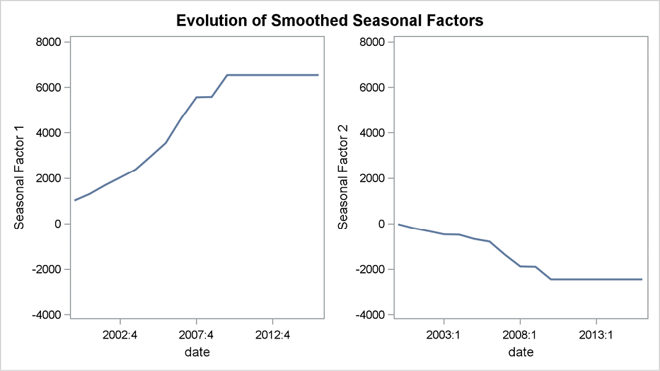
Figure 12.7 Seasonal component for second and third quarter

12.2 Regression Components
In the following application, the various possibilities offered by PROC UCM for inclusion of regression terms in the model are demonstrated. The total retail sales is included as an independent variable when modeling the volume of e-commerce. In a first attempt, shown in Program 12.2, the independent variable is included with a constant regression coefficient, as in usual linear regression models. The independent variable is simply specified in the MODEL statement. Of course, more than one independent variable could be included by the same syntax, as with other regression procedures in SAS.
Program 12.2 Including an independent regression variable in PROC UCM
ods graphics;
PROC UCM data=sasts.E_commerce;
id date interval=quarter;
model E_commerce=Total_retail;
level plot=smooth;
slope plot=smooth var=0 noest;
season length=4 plot=smooth;
outlier ;
estimate plot=(panel residual);
forecast lead=24 plot=forecasts alpha=0.1;
run;
ods graphics off;
Output 12.4 Estimated regression coefficient and component variances

The regression coefficient is estimated along with the component variances; see Output 12.4. The value, 0.039, is clearly significant as shown in the table of parameter estimates. It indicates that the volume of e-commerce corresponds to about 4% of the total retail value. The slope component is estimated as a constant because the variance for this component is fixed at 0. The value of the slope is given in Output 12.5 as 633, which is a bit below the value 850 in the model without the independent variable, as seen in Output 12.3. Because the slope component in this model describes the increasing importance of e-commerce, the regression describes only the part of e-commerce that is proportional to the total retail sales. This part could be due to inflation, economic growth, or other factors affecting the two series in the same way. This regression then explains why the slope is reduced from a steady increment of 850 billion dollars to just 633 billion dollars. The seasonal component in this model specification allows for different seasonal structures of e-commerce and total retail sales. Similarly, the significant upward trend corresponds to the more rapid increase in e-commerce compared to total retail sales.
Output 12.5 Estimated level and slope component for the last observation for a completely fixed slope

Obviously, the model has to take into account the fact that e-commerce in the observation period has increased in importance relative to the value of total retail sales. This fact can be included in the model if the regression coefficient is allowed to be time varying. This is obtained by using the RAMDOMREG statement in Program 12.3 as an alternative to the fixed regression specified in the MODEL statement in Program 12.2. The level is fixed by setting its variance to 0, in order to avoid over-parameterizations, and no slope component is included. The trend is described only by the independent variable, the total retail sales, which is upward trending. The increasing importance of e-commerce is now described by the time-varying regression coefficient.
Program 12.3 Allowing for a time-varying regression coefficient in PROC UCM
ods graphics;
PROC UCM data=sasts.E_commerce;
id date interval=quarter;
model E_commerce;
randomreg Total_retail /plot=smooth;
level plot=smooth var=0 noest;
season length=4 plot=smooth;
outlier ;
estimate plot=(panel residual);
forecast lead=24 plot=forecasts alpha=0.1;
run;
ods graphics off;
The smoothed version of the time-varying regression coefficient is plotted by the plot=smooth option. Note that this option must be preceded by a slash (/) in the RANDOMREG statement, but no slashes are needed for the options in the LEVEL, SLOPE, or SEASON statements. The plot of the regression coefficient, Figure 12.8, shows that the coefficient has increased from 0.03 (that is, 3% of the total retail sales) in the year 2000 to 0.06 in 2010. If a slope component is included in the code, the regression coefficient becomes more constant, with values rising only from 0.036 to 0.040.
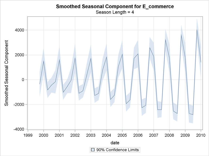
The seasonal component, shown in Figure 12.9, changes over the years. In fact, the seasonal spike has moved from the first quarter to the fourth quarter of the year. Keep in mind that the seasonality in this model is not for the value of e-commerce itself but for the residuals in the regression using total retail sales as an input variable. This means that the interpretation of Figure 12.9 is different from the interpretations of Figures 12.6 and 12.7. One possible explanation for these differing interpretations is problems in tracking the volume of e-commerce. In recent years, the time that the actual trade is observed reflects the time that it was actually made, whereas in previous years, e-commerce that is attributable to Christmas sales might not have registered until the beginning of the next year.
Figure 12.8 The time-varying regression coefficient

Figure 12.9 The seasonal component in the model with a time varying-regression coefficient
12.3 Model Fit
The residuals are plotted along with a panel of diagnostic plots for model fit, as specified by the plot=(panel residual) option in the ESTIMATE statement. (See Figures 12.10 and 12.11.) The model fit seems acceptable when judged from the panel of residual plots, because no autocorrelation problems appear to be present. Also, the normality assumption seems acceptable.
Figure 12.10 One quarter ahead forecast errors
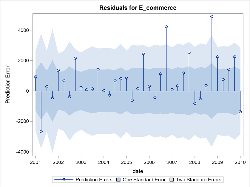
Figure 12.11 Diagnostic plots for model fit

The residual plot, Figure 12.10, might indicate some heteroscedasticity problems because the variance of the residuals seems to increase over the years. The residual for the second observation is numerically large, but this is probably due to burn-in problems and is not of any econometric importance. The estimated seasonal component has an increasing amplitude, which also indicates heteroscedasticity. (See Figure 12.9.) This is, however, natural. It is more realistic to describe residuals and seasonality as relative features and not in absolute terms.
In most econometric modeling, this increasing variation would call for a logarithmic transformation. However, PROC UCM offers no multiplicative version or other transformation possibilities like PROC ESM does for exponential smoothing and PROC X12 does for seasonal adjustment. In applications of PROC UCM, the only possibility for multiplicity modeling is to model the logarithmically transformed series, followed by a transform back again by the exponential function.
All the time-varying components, coefficients, and so on in PROC UCM to a large extent make such transformations superfluous in model building, as demonstrated in the applications in this section. Allowing every part of the model to evolve over time makes homogeneity and stationarity conditions unnecessary in the process of finding useful results. Also, in many situations, results are needed in the original scale. The results obtained by a log transformation and a transformation back by exponentials are hard to communicate to a non-mathematical audience, which usually demands only results.
For this reason, PROC UCM is a safe choice if you need results but you don’t want to end up with a genuine statistical modeling that is thoroughly tested. Moreover, the easy coding and the rich number of graphics produced are very attractive features of PROC UCM