Chapter 13: An Analysis of the Arctic Ice Coverage Series Using Unobserved Components

13.1 The Time Series

13.2 Aggregation to Yearly Averages

13.3 Aggregation to Monthly Averages

13.4 Aggregation to Weekly Averages

13.5 Aggregation to a Series Observed Every Second Day

13.6 Analysis of the Daily Series

13.7 Concluding Remarks

13.1 The Time Series

In this chapter, the idea of unobserved components models is applied to a series of observations of the total ice coverage in the Arctic Ocean. This series contains observations made every second day from November 1, 1978, to August 19, 1987. After that date, it contains observations made daily up to the end of 2007. The series is aggregated to many levels in order to demonstrate the various possibilities offered by PROC UCM. The aggregation is performed using PROC TIMESERIES, as described in Section 3.2, but the very short code is repeated in order to make it clear which aggregation level is being applied for each call of PROC UCM.

13.2 Aggregation to Yearly Averages

In Program 13.1, the series is aggregated to yearly averages by applying PROC TIMESERIES. Because ice coverage data for only the last two months of 1978 is available, it is impossible to calculate the average ice coverage for the full year of 1978. In the application of PROC TIMESERIES, this implies that observations previous to January 1, 1979 are deleted by the WHERE statement, in which the flexibility of the SAS facilities for handling date variables is demonstrated. The final series of yearly averages includes data for the years 1979–2007, yielding a total of 29 observations.

An ID statement is required with PROC UCM in order to specify the time variable, which should be a SAS date time variable. Moreover, you should specify the interval in the correct SAS notation for such intervals. The application of PROC UCM in Program 13.1 fits a model with both a time-varying level component and a time-varying slope component, using the model described in Section 10.2. The smoothed versions of the fitted level and slope components are plotted. The option plot=(residual panel) in the ESTIMATE statement results in a plot of the time series formed by the residuals, a panel plot of residual autocorrelations, and a histogram and a normal probability plot of the residuals.

Program 13.1 PROC UCM applied to the yearly aggregated ice coverage series

PROC TIMESERIES data=sasts.Arctic_ice_daily out=Arctic_ice_yearly;
id date interval=year accumulate=average;
var _numeric_;
where date > ‘31dec1978’d;
run;
				
ods graphics;
PROC UCM data=Arctic_ice_yearly;
id date interval=year;
model Total_Arctic;
level plot=smooth;
slope plot=smooth;
estimate plot=(residual panel);
forecast lead=10 plot=all alpha=0.1;
run;
ods graphics off;

The estimated variances of the remainder terms for two fitted components are printed in the text output; see Output 13.1. The error variance of the slope component is very close to 0, which means that the slope coefficient is almost constant for the whole time period. The error term of the level component is rather large because the level varies during the observation period.

Output 13.1 Estimates for the level and slope component variance

For this reason, the slope parameter is fixed by the options variance=0 and noest in the SLOPE statement.

slope plot=smooth variance=0 noest;

Figure 13.1 Forecasts in a model with a fixed slope parameter

In this application, the variance of the level component is significantly positive, and the level component follows the observed series with only small residuals. In order to give an idea of the model fit, the forecast plot is specified in the FORECAST statement. The forecasts are plotted with 90% confidence limits by the option alpha=0.1 instead of with the default 95% confidence; see Figure 13.1. The model structure is dominated by the negative trend, which is also apparent in the forecasting period. In the printed output, the estimate of the slope component appears; see Output 13.2. Because this value is about one and a half times its standard deviation, the slope is insignificant, but this might be due to the rather small number of observations.

Output 13.2 The level and slope component estimated for the last observation

Figure 13.2 The model fit for the model with a fixed slope parameter

The panel plot for judging the model fit, Figure 13.2, clearly shows that an autocorrelation problem exists because the first-order autocorrelation is significantly negative. Such autocorrelations can be modeled in many ways by PROC UCM, and in this chapter a variety of these are demonstrated. One possibility is to overlay the model with an autoregressive component using an AUTOREG statement. However, this introduces a new stochastic component into the model, which is one too many for such a short series. Therefore, it is preferable to also fix the level component as a constant value by fixing its variance at 0. The resulting code is seen in Program 13.2.

Program 13.2 Including an autoregressive component in the application for yearly aggregated series

ods graphics;
PROC UCM data=Arctic_ice_yearly;
id date interval=year;
model Total_Arctic;
autoreg  plot=smooth;
level plot=smooth variance=0 noest;
slope plot=smooth variance=0 noest;
estimate plot=all;
forecast lead=10 plot=all alpha=0.1;
run;
ods graphics off;

For both the ESTIMATE and the FORECAST statements, all available plots are constructed. One example is the smoothed trend plot, shown in Figure 13.3, which plots the observations and the level/slope component, which is continued in the forecasting period. The negative trend is clearly visible and the fit seems reasonable, but for the last three observations the trend appears to be steeper than in the beginning of the observation period. In the first attempt to model the trend, a time-varying slope is used because the trend seems to vary. But only three observations are too few to catch a new trend. For this reason, in the model allowing for both a time-varying level and slope, these three observations were modeled by the level component and not by the changing slope parameter.

The autoregressive component is plotted in Figure 13.4. The autoregressive parameter is estimated as 0.35. This is positive in order to fit the systematic behavior in the sign of the residuals, such as the many positive residuals for the years 1997 to 2004 and the negative residuals for the last three observations.

Figure 13.3 The fixed trend estimated in the model with an autoregressive component

Figure 13.4 The estimated autoregressive component

This model structure is different from the first model. Both the level and the slope component are fixed, leaving the autoregressive component as the only stochastic element in the model. This component is stationary, which is the reason for the much shorter confidence intervals in Figure 13.5. Although the successive addition of innovation terms in the dynamic specification in Program 13.1 leads to infinitely increasing forecast variances in Figure 13.1 for large forecasting horizons, the forecasting variance has an upper limit for the stationary component. See Figure 13.5, which also shows the effect of the autoregression as a small curvature of the forecast function.

Figure 13.5 Forecasts in the model with an autoregressive component

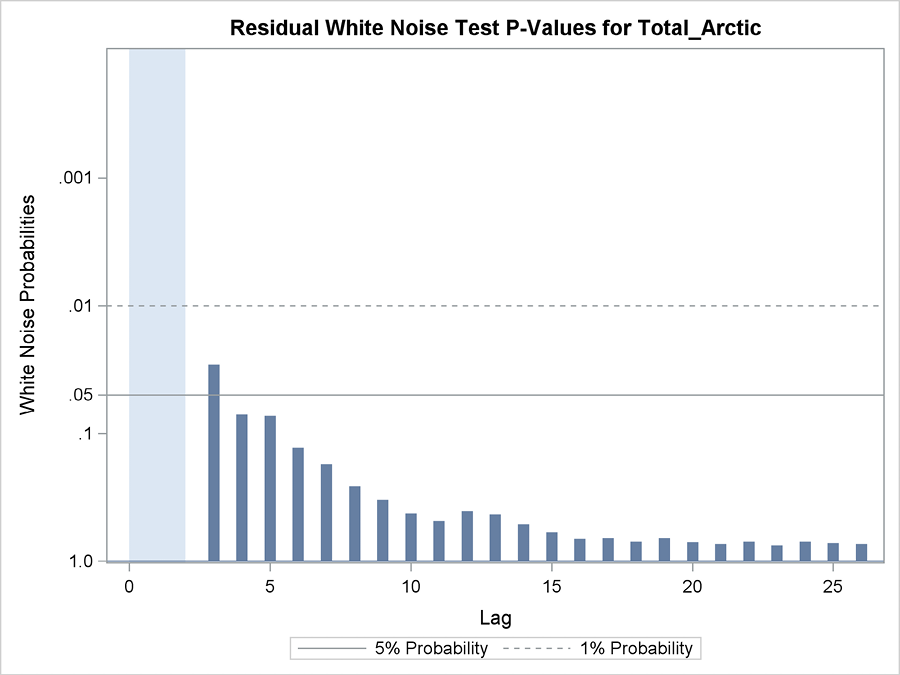
The autocorrelation problem is solved by adding the component. Among the many plots specified by the plot=all option in the ESTIMATE statement is a plot for white noise tests for the hypothesis that the autocorrelations in the residual series for each separate lag are 0 (see Figure 13.6). These tests all have p-values above 10%, because all estimated autocorrelations are below the 0.1 horizontal line. Note that the lag 1 and 2 residual autocorrelations are excluded from the testing, indicated by the shaded portion of the graph. The reason for this is that the fitted autoregressive model is designed to account for these autocorrelations.

Figure 13.6 Test p-values for zero autocorrelations

13.3 Aggregation to Monthly Averages

In Program 13.3, the observed series is first aggregated to a series of monthly averages by PROC TIMESERIES, and afterward PROC UCM is applied for the resulting monthly series. The level of integration is specified by the option interval=month in the ID statement, along with the name of the time index variable date. A seasonal component has to be included in the model. The parameters of the seasonal component are fixed because the variance is set to 0 by the options var=0 and noest. Moreover, both the level and the slope are fixed so that the only stochastic component is an irregular component. The model is a sum of a trend line and fixed monthly dummy parameters with an added series of independent, identically distributed variables. The parameters for the trend line and the seasonal dummies are estimated from data. This irregular component in this model is, however, not the same as remainder terms in a usual regression setup, so residuals are also present.

Program 13.3 PROC UCM applied to the monthly aggregated series of Arctic ice coverage

PROC TIMESERIES data=sasts.Arctic_ice_daily out=Arctic_ice_monthly;
id date interval=month accumulate=average;
var _numeric_;
run;

ods graphics;
PROC UCM data=Arctic_ice_monthly plots=all;
id date interval=month;
model Total_Arctic;
irregular;
level  var=0 noest;
slope var=0 noest;
season length=12 print=smooth var=0 noest;
estimate extradiffuse=3;
forecast lead=120 plot=all alpha=0.1;
run;
ods graphics off;

The variance of the irregular component is printed in the table of estimates for free parameters. The fixed level and slope parameters are printed in the table of states for the last observation in the observation period. These tables are shown in Output 13.3. Because these parameters are constant for all observations, these values can be considered as estimated parameters, with standard deviations also provided in the output. The negative slope is highly significant. Because this slope is constant, the smoothed slope plot, requested with all the other plots, is just a straight horizontal line, which is, of course, non-informative.

Output 13.3 Estimates in the model with an irregular component and fixed level and slope components

The seasonal component is simply 12 dummy parameters that are printed in the text output by the print=smooth option. Output 13.4 includes the first 12 values because the numbers for the remaining observations are simple repetitions. These 12 estimates are repeated in the text output for each year. They are also plotted, but because the whole observation period is rather long, the horizontal axis is too short to see any details in the plot. The 12 seasonal dummies for a year sum to 0. Otherwise, the seasonal component would affect the level and slope components.

Output 13.4 The estimated fixed seasonal component

In Program 13.3, all available plots are constructed by the plots=all option in the procedure call. Many of these plots tell the same story in different ways (for example, that the ice coverage is declining and that the series contains a major seasonal component). This is visible in the trend plot, Figure 13.7. This plot shows the trend line and the observed values, which differ from the trend line in a systematic way due to the seasonal variation.

Figure 13.7 The trend in a model for monthly data with a clear seasonal pattern

The option extradiffuse=3 in the ESTIMATE statement excludes the first three residuals from the residual plot and from the residual diagnostic testing. This is because these first residuals are made dubious by the fact that the estimation procedure is unable to adapt to the real situation after only a few observations. Depending on the situation, however, another reason for this exclusion might be that the first observations are measured with a larger variation than the rest of the series. For this series, these first three residuals are numerically large, and their standard deviations are so large that they disturb the model testing. Also, it is impossible to judge the model fit by the provided plots because the vertical axis simply becomes too long to fit huge confidence limits for these residuals.

The residual plot, Figure 13.8, with the first three residuals excluded, provides a messy picture. The series is long, but the main finding is that the last residuals are remarkably negative, meaning that the trend cannot catch the more accelerating de-icing for the last years of the observation period. For the distribution of the residuals, these large negative values lead to a heavy left tail, which is clearly seen in the probability plot at the upper left corner in the residual panel plot, Figure 13.9. The distribution therefore is non-normal.

Another finding from the residual plot (Figure 13.8) is that the signs of the residuals are to some extent systematic, because many consecutive residuals have the same sign. This is to be expected. It is common for some winters to be cold while others are warm, leading to either major or minor ice coverage for many consecutive months.

These phenomena are statistically explained by the notion of autocorrelation, meaning that residuals for neighboring months are positively correlated. The autocorrelation plot is shown in the residual panel plots in Figure 13.9. The autocorrelation function in the lower left corner of the panel shows exponentially decaying autocorrelations. The partial autocorrelation function in the lower right corner shows a distinctive first-order partial autocorrelation with a value of about 0.7– 0.8. The remaining partial autocorrelations seem insignificant. This behavior is the standard picture for identification of a first-order autoregressive model, AR(1), as also described in Chapter 7. The second-order partial autocorrelation might also be significant. Combined with the cycling behavior in the overall picture for the autocorrelation function, this might indicate that a second-order autoregression, AR(2), is an even better model.

Figure 13.8 One-step-ahead forecast errors for the model in Program 13.3

Figure 13.9 Plots for model fit

Because the model includes an irregular component, a simple possibility is to specify this component as an autoregressive noise series instead of as a component of independent random terms on top of the other model components. The second-order autoregressive model is specified by the option p=2 in the IRREGULAR statement.

irregular p=2;

All seasonal ARMA models could specify the irregular component in this way. By these facilities PROC UCM can be seen as an alternative to the other econometric time series procedures in SAS, such as PROC AUTOREG, PROC ARIMA, and PROC VARMAX. The ARMA(0,1)×ARMA12(0,1) for the stationary part of the airline mode is specified by the IRREGULAR statement in the following code. The differences in the full airline model ARMA(0,1,1)×ARMA12(0,1,1) are specified by the DEPLAG statement. See Chapter 7.

deplag lags=(1)(12) phi=1 1 noest;

irregular q=1 sq=1 s=12;

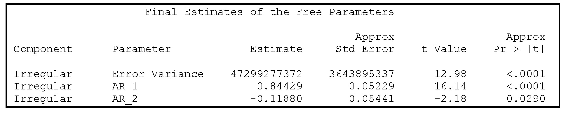
The estimated second-order parameter is significant when tested at a 5% level, but the numerical value is close to 0, so, in practice, it makes no difference to the model fit whether this term is included. See Output 13.5.

Output 13.5 Estimates for the AR(2) irregular component

For the model with only a first order autoregressive term, specified by the option p=1, the autocorrelation test shows some significance at lag 1, but not for a 1% test level, and for the remaining lags the fit is accepted. See Figure 13.10.

Figure 13.10 Testing for zero residual autocorrelations in a model with an AR(1) term

13.4 Aggregation to Weekly Averages

For weekly data, seasonality is of course also present. However, the seasonal specification by dummy variables, which was applied for the monthly data, requires the estimation of 52 parameters, one for each week of the year. This could be accomplished as in Program 13.4. The resulting seasonal structure consists of an estimated value for each week in the data period where the form seems very regular, like a sinusoid. It seems clear that the number of free parameters can easily be reduced by use of this regularity. See Figure 13.11.

Program 13.4 PROC UCM applied to the weekly aggregated series of Arctic ice coverage

PROC TIMESERIES data=sasts.Arctic_ice_daily out=Arctic_ice_weekly;
id date interval=week accumulate=average;
var _numeric_;
run;

ods graphics;
PROC UCM data=Arctic_ice_weekly plots=all;
id date interval=week;
model Total_Arctic;
irregular ;
level var=0 noest;
slope var=0 noest;
season length=52  ;
estimate;
run;
ods graphics off;

Figure 13.11 The estimated seasonal component, consisting of 52 weekly dummies

The alternative parameterization of the seasonal component by sinusoids is often useful for time series with a seasonal behavior that depends only on meteorological conditions. Under the assumption that a year consists of exactly 52 weeks, you can mathematically establish that every seasonal dummy model is equivalent to a model that includes sinusoids with various periods that form the harmonics of a 52-week seasonal length. The harmonics have period lengths 52, 52/2, 52/3, 52/4, .. , 2. These sinusoids consist of a cosine and a sine with different coefficients. In PROC UCM, a seasonal component can be parameterized by the SEASON statement using sinusoids. The number of estimated parameters can be dramatically reduced by including only a few of these harmonics.

Other series with seasonal behavior due to human activity, such as the volume of e-commerce, include seasonality due to activity that is completely independent of weather conditions (for example, buying that occurs around Christmas). In these cases, the parameterization by sinusoids might require too many harmonics, making this specification of the seasonal less attractive. If weekly data includes such seasonals apart from meteorological seasonality (for example, an effect of Valentine’s Day), they can be included in the model by using independent variables in regression-type models. The rest of the seasonal variation could be parameterized using just a few sinusoids.

Program 13.5 Coding a parameterization of a seasonal variation by harmonics

PROC TIMESERIES data=sasts.Arctic_ice_daily out=Arctic_ice_weekly;
id date interval=week accumulate=average;
var _numeric_;
run;
				
ods graphics;
PROC UCM data=Arctic_ice_weekly plots=all;
id date interval=week;
model Total_Arctic;
irregular ;
level var=0 noest;
slope var=0 noest;
season length=52 type=trig print=harmonics ;
estimate;
run;
ods graphics off;

For the weekly data series, a seasonal component using sinusoids is specified in Program 13.5 under the unrealistic assumption that a year consists of exactly 52 weeks. In this code, the weight for all harmonics—period lengths—are printed. The result is that only 1 and 2, and maybe number 5, are significant. See Output 13.6. Only the first two harmonics are included in the model with the keeph parameter by the statement

season length=52 type=trig print=harmonics keeph=1 2;

in order to reduce the number of parameters (keeph is derived from “keep harmonics”).

Output 13.6 Estimates for all harmonic components for weekly the aggregated series

Another problem is that the seasonal length is not an integer number. A year in precise terms lasts 365.24 days, so the number of weeks according to astronomy is 365.24/7 = 52.18, which is a non-integer. This can be accounted for by applying a cycle component instead of a seasonal component in order to parameterize seasonality in the form of harmonic sinusoids, as in this series. The basic version is simply to apply one CYCLE statement in PROC UCM without options for period length, and so on. Printing and plotting options are necessary, of course, but to do the job, only one word is necessary:

cycle;

In the printed output, the period length, the damping factor, and a component variance are printed, along with the other model parameters for level and slope, for example. See Output 13.7.

Output 13.7 Estimates for a model with a single cyclic component

It is remarkable that the period length is very close to the exact number of weeks per year. In this way, it is possible to test the hypothesis of 52 weeks per year, even though this is of course ridiculous. In order to include all available knowledge in the model, this fact should be used as a fixed number and not as a stochastic element. In the next application of PROC UCM, the period length is fixed to the exact value 365.24/7 = 52.18 by a noest option in the CYCLE statement in order to specify which parameter is excluded from the estimation algorithm.

cycle period=52.18 noest=period;

The estimated damping factor is very close to 1 and is, in fact, insignificantly different from one. This is in accordance with the hypothesis that the effect of the yearly variation depends on heating from the sun, which has a constant seasonal variation due to the rotation of the earth. But it is also possible that the seasonal effect is proportional to the ice coverage because the ice coverage is measured in absolute terms but the ice coverage is also declining during the observation period. In unobserved component models, this leads to a damping factor of less than 1.

The damping factor is fixed to the number 1 by excluding one more parameter from the estimation.

cycle period=52.18 rho=1 noest=(rho period);

The cycle component variance also seems to be insignificant, indicating that the seasonal structure is fixed and not time-varying, which is rather natural in the context. The results in Output 13.8 are based on a completely fixed cycle component by:

cycle period=52.18 rho=1 variance=0 noest=(rho period variance);

It is possible to include many cycle components in applications of PROC UCM. If one more cycle is included without any restrictions, the second-order harmonic, half a year, is in fact nearly replicated because the period length is estimated to be around 28 weeks. A more healthy procedure is to fix this cycle to the correct period length, which is half the number of weeks per year (26.09). The cycle components are then specified to obtain the same results as the code, using the trigonometric parameterizations in the SEASON statement with just two harmonics but with a better period length more in accordance with the exact physical conditions.

cycle period=52.18 rho=1 variance=0 noest=(rho period variance);

cycle period=26.09 rho=1 variance=0 noest=(rho period variance);  

In this model, autocorrelation problems exist. In order to demonstrate the wide range of facilities in PROC UCM, these problems are remedied in Program 13.6 by a DEPLAG statement. With this statement a lagged value of the observed series is included as an independent variable in the model. Also in this code, a first-order autoregressive model is used for the irregular component. The estimated parameters are shown in Output 13.8.

Program 13.6 Introducing a lagged variable in a model for weekly observations of ice coverage

ods graphics;
PROC UCM data=Arctic_ice_weekly plots=all;
id date interval=week;
model Total_Arctic;
deplag lag=1;
irregular p=1;
level var=0 noest;
slope var=0 noest;
cycle period=52.18 rho=1 variance=0 noest=(rho period variance);
cycle period=26.09 rho=1 variance=0 noest=(rho period variance);
estimate;
run;
ods graphics off;

Output 13.8 Estimates for the model specified by Program 13.6

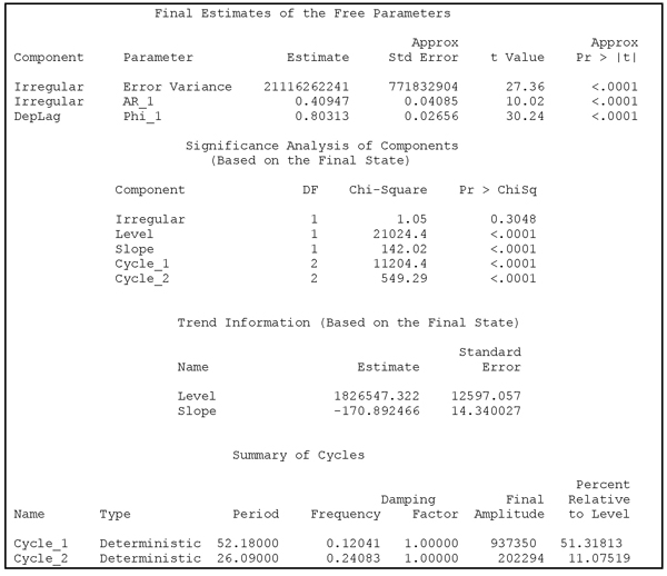
The residual panel, Figure 13.12, shows that the autocorrelations are close to 0 and that the residuals are closely described by the normal distribution.

Figure 13.12 The model fit for the model with two cyclic components for the weekly aggregated series

13.5 Aggregation to a Series Observed Every Second Day

The series is observed every second day for the first part of the observation series. An aggregation to a series observed every second day is the highest frequency possible without interpolation. In Program 13.7, this aggregation is obtained by an application of PROC TIMESERIES using the aggregation level day2, which in the SAS naming convention means every second day. In PROC UCM, the interval between observations is also denoted day2 in the specification of the interval between consecutive observations in the ID statement. As in the application for weekly data, seasonality is modeled by two cycles with fixed period lengths that correspond to one year and a half year. For a series of observations every second day, a full yearly cycle has the length 365.24/2 = 182.62 and a half year 365.24/4 = 91.31. The variances in the cycle statements are set to 0, so the amplitudes are estimated as constant numbers instead of as time-varying components. Note that now all three parameters of the cycles are excluded from the estimations. Moreover, autocorrelations are included in the model specification by a first-order autoregressive model for the irregular component. The code is shown in Program 13.7.

Program 13.7 Analyzing the series of ice coverage aggregated to every second day

PROC TIMESERIES data=sasts.Arctic_ice_daily out=Arctic_ice_day2;
id date interval=day2 accumulate=average;
var _numeric_;
run;
ods graphics;
PROC UCM data=Arctic_ice_day2 plots=all;
id date interval=day2;
model Total_Arctic;
irregular p=1;
level var=0 noest ;
slope ;
cycle period=182.62 rho=1 variance=0 noest=(rho period variance) ;
cycle period=91.31 rho=1 variance=0 noest=(rho period variance);
estimate;
run;
ods graphics off;

The total fit is best displayed by the smoothed level plot, Figure 13.13. The model has a time-varying slope because this parameter is not restricted to a constant by fixing its variance at 0. This is successful for this aggregation level because the number of observations is larger than for the previous yearly or monthly data series. The slope coefficient becomes increasingly negative, as seen in Figure 13.14, as the downward trend accelerates at Figure 13.13. The autocorrelation plots show that some autocorrelation is present in the residual series, but if an additional lag is introduced by letting p=2, the estimation algorithm becomes unstable.

Figure 13.13 The level component extracted from a series of every-second-day observations

Figure 13.14 The time varying slope component for the series of every-second-day observations

13.6 Analysis of the Daily Series

In this section, daily observations for the whole observation period are analyzed. First, the series is aggregated (or, rather, interpolated) from observations every second day to daily observations in the first part of the observation period by applying PROC TIMESERIES or PROC EXPAND. Of course, it is somewhat specious to guess unobserved values, but interpolation is possible by various algorithms, as was described in more detail in Chapter 4.

In the first application, shown in Program 13.8, the aggregation is done by simple averages using PROC TIMESERIES. Because it is impossible to calculate an average for a day without any observation, these days are set to missing in the output data set. But PROC UCM allows for missing values as long the variable in the ID statement, here the variable date, is present for all days. In this way, the number of observations in the data set is 10653, but, because 1607 observations are missing, the real number of observations is 9046. Note that this application uses only observed values, and no interpolation leading to homemade observations is applied.

Program 13.8 PROC UCM applied to all available observations

PROC TIMESERIES data=sasts.Arctic_ice_daily out=Arctic_ice_day1;
id date interval=day accumulate=average;
var _numeric_;
run;
				
ods graphics;
PROC UCM data=Arctic_ice_day1 plots=all;
id date interval=day;
model Total_Arctic;
irregular p=2;
level var=0 noest ;
slope ;
cycle period=365.24 rho=1 variance=0 noest=(rho period variance);
cycle period=182.62 rho=1 variance=0 noest=(rho period variance) ;
estimate;
forecast lead=3650;
run;
ods graphics off;

Another possibility is to interpolate the missing observations by PROC EXPAND, as done in Program 13.9. By default, this interpolation is done by fitting a spline function to the observed values and then predicting the missing observations along this curve. From the viewpoint of a times series analysis, this is yet another type of smoothing of the observed series. The resulting series should be smoother on a day-to-day basis than the original series (even though the original series is unobserved). In the model fitting, this implies that the irregular component and the innovation variances in fitted components become less important.

It turns out that the estimation algorithm becomes unstable, leading to a nonstationary solution for the autoregressive parameters. For this reason, initial values (the estimates from Program 13.8) for the autoregressive parameters in Program 13.9 are specified in the IRREGULAR statement in order to improve the convergence of the estimation.

Program 13.9 Interpolating the ice coverage to daily observations

PROC EXPAND data=sasts.Arctic_ice_daily out=Arctic_ice_day1_spline to=day;
id date;
run;
				
ods graphics;
PROC UCM data=Arctic_ice_day1_spline plots=all;
id date interval=day;
model Total_Arctic;
irregular p=2 ar=1.26 -0.28;
level var=0 noest ;
slope ;
cycle period=365.24 rho=1 variance=0 noest=(rho period variance);
cycle period=182.62 rho=1 variance=0 noest=(rho period variance) ;
estimate;
run;
ods graphics off;

The results from Program 13.8 and Program 13.9 are very similar. The number of observations is large, and the execution time is long, especially as all available plots are requested by the option plots=all in the procedure call. But it is possible to extract a meaningful overall level component that is dominated by the negative trend. Figure 13.15 presents the level based on Program 13.8 without interpolated observations. The same trend plot is more “fluffy” for the estimates that use interpolation, as in Program 13.9.

Figure 13.15 The estimated level component from the series of all available daily observations

The residuals seem to be well described by the normal distribution, although there are a few outliers shown in the residual diagnostic panel in Figure 13.16. The autocorrelations are small but nevertheless significant because the number of observations is very large. The plot of the residual series, Figure 13.17, clearly shows that the variance is smaller after 1987 than before. This must be due to the change in observation frequency from every second day to every day.

Figure 13.16 Model fit for the model for all available daily observations

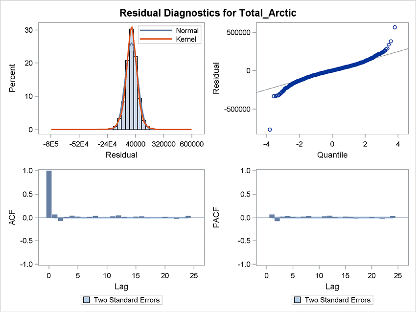
Figure 13.17 Daily one-step-ahead forecasts errors

Output 13.9 Outliers in the model for daily data

The three most important outliers are from September 1984; see Output 13.9. They can easily be deleted from the input data set because PROC UCM allows for missing observations, as seen in Program 13.10. Another possibility is to replace these outliers with interpolated values using PROC EXPAND. In this situation, suppressing the outliers in other ways does nothing to change the resulting estimates. It turns out that the algorithms underlying these unobserved component models are robust toward outliers, at least for a long time series such as this one.

Program 13.10 Deleting outliers

data a;
set sasts.Arctic_ice_daily;
if date>’11sep1984’d and date<’17sep1984’d then Total_Arctic=.;
run;
PROC TIMESERIES data=a out=Arctic_ice_day1;
id date interval=day accumulate=average;
var _numeric_;
run;
ods graphics;
PROC UCM data= Arctic_ice_day1 plots=all;
id date interval=day;
model Total_Arctic;
irregular p=2 ar=1.26 -0.28;
level var=0 noest;
slope ;
cycle period=365.24 rho=1 variance=0 noest=(rho period variance);
cycle period=182.62 rho=1 variance=0 noest=(rho period variance) ;
estimate ;
forecast lead=3650;
run;
ods graphics off;

13.7 Concluding Remarks

In this chapter, PROC UCM is applied to many aggregation levels of the same series. For this particular series, the long-term properties of the ice coverage are probably the most interesting subject. This means that the ability to extract a meaningful level and trend from the data is the most important outcome of the analysis. However, the series is too short when aggregated to just yearly observations, and the resulting estimated trend curve is unsatisfactory.

When aggregating to higher frequencies, the number of observations increases but at the expense of seasonality appearing as an extra problem. For monthly data, this seasonality can be successfully modeled by dummy variables. This method extracts a meaningful trend curve from the data series because it is based on more observations of the seasonal adjusted data monthly series instead of on the yearly series.

When aggregation is performed on weekly data, it seems unrealistic to estimate seasonal weekly dummies because the number of weeks each year is high. This appears to lead to too many parameters, but in practice, the results seem acceptable. Another problem is that the number of weeks in a year is not a constant integer, making a parameterization by sinusoids seem more attractive. One possibility is to model the seasonality by sinusoids because the weather conditions underlying the seasonality are stable from year to year and are very regular, depending on the angle of the sun over the horizon at midday during the year. In either case, the extracted trend curve is realistic, and the forecast plot of the series of weekly observations and the fitted trend curve clearly show that a well-defined trend is found in the wilderness.

When aggregating to observations every second day or every day, the estimations become unstable, and the results of some of the estimations are misleading. This might be due to outliers or a lack of machine resources, but most of the problems can be fixed by clever initialization of parameters for the iterative estimation algorithm or by fixing some of the parameters at reasonable numbers.

For aggregated levels, outliers are smoothed. They are constructed by averages and for that reason, they do not present problems. Outliers are more important for highly frequent series.

If the purpose of the analysis is to study the long-term behavior of the ice coverage, then short-term dynamics for daily data is of no importance at all. This means that solving problems in estimating, for example, autoregressive models for the residuals of the long-term models is useless. So the desire to obtain a final model with an acceptable fit in all aspects is too ambitious. As demonstrated, the methods behind these unobserved component models are robust for short-term events like outliers in the series. They also result in the reasonable estimation of the trend and level, even if the resulting model is invalid in some dimensions.