Chapter 7. Maximizing Mondrian performance

This chapter is recommended for

	Business analysts
	Data architects
	Enterprise architects
	Application developers

Adventure Works analysts have been generally happy with the Mondrian’s abilities. They like the reports and dashboards and particularly being able to do analysis on the fly. Some have even become proficient with MDX queries for performing advanced analysis. But as the amount of data grows, some of the reports and analyses are starting to feel sluggish, and not as quick as users demand.

One of the promises of Mondrian is that it supports analytics at the speed of thought. This means that when an analyst makes changes to a report, such as adding or removing dimensions and measures, adding calculations, and applying filters, the report needs to be updated within seconds, rather than minutes or hours. Given that analysis is often done over millions of records, performance is extremely important.

Out of the box, with a well-designed star schema, Mondrian performance is very good for a wide variety of datasets and queries. But some businesses want to do real-time analysis against millions of facts and thousands of dimension members. Eventually, even the fastest database and software will start to bog down with straight database calls. By default, Mondrian will perform some caching to speed things up, but squeezing out the highest levels of performance from your data sometimes takes additional configuration and effort.

There are three main strategies for increasing performance: tuning the database, aggregate tables, and caching. This chapter will discuss how to tune Mondrian using all three approaches. By the end of this chapter, you’ll understand the techniques you can use to optimize Mondrian performance and keep the analytics flowing smoothly.

7.1. Figuring out where the problems are

Performance is something that you’ll want to consider early on. While performance may appear to be fine with small test sets, problems can show up when the amount of data gets large. Some of the possible solutions, such as using aggregation tables, additional servers, and even a different database can be extremely costly and challenging to implement after the system has gone live. This section will present a general process for testing performance and then describe the necessary steps to prepare for performance testing and improvement.

7.1.1. Performance improvement process

You can start evaluating performance with any part of the system, but experience has identified a general approach that works best for most Mondrian deployments. Each step in this process has the potential to improve performance, with the early steps usually providing the largest performance gains.

Figure 7.1 shows the high-level process for this performance improvement.

Figure 7.1. Performance improvement process

There are five high-level steps to perform when evaluating Mondrian’s performance. Figure 7.1 and the following list show the order of analysis, but the order in which you implement solutions may vary. Either way, you can’t go wrong following these steps.

1.  First, prepare for performance testing. Section 7.1.2 covers the general considerations when preparing for performance testing, such as setting up the test environment and preparing data.

2.  Once you’re set up, you need to evaluate the current performance. “Executing the queries” in section 7.1.2 covers this topic, but it essentially involves running queries in your test environment.

3.  If the performance isn’t satisfactory, it’s best to start analysis and tuning with the database, as described in section 7.2

4.  If tuning the database doesn’t solve your performance problems, you’ll want to tune your Mondrian schema. Later sections on aggregate tables and caching will show how to speed up your queries.

5.  Finally, if you’ve done all the tuning you can and are still unhappy with the performance, you should look for alternative ways of presenting the information, such as breaking up the data into different cubes or doing analysis with preset filters. These topics aren’t covered directly in this book.

It might be the something else

There are other possible reasons for poor performance, beyond those given here. For example, poor network latency between Mondrian and the database can slow down the system. The system running the Mondrian engine might also be underpowered. To eliminate these variables, it’s often ideal to initially do performance testing in a confined environment.

7.1.2. Preparing for performance analysis and establishing current performance

This section will cover the first two steps of the tuning process shown in figure 7.1. Before you can start your analysis, you need to have an environment, a baseline of test data, and a set of queries to run. It’s helpful to have a dedicated environment for testing that’s separate from the development environment. Although any improvement helps, some of the tuning that you may want to do involves creating a cluster of servers, which is something not typically found in a development environment.

Figure 7.2 shows what a performance test environment might look like.

Figure 7.2. Performance test environment

Hardware and software environment

First you need the hardware environment and software set up for testing. This architecture should look a lot like what you want your production environment to look like. For instance, suppose you plan on running the data warehouse databases on a separate server from Mondrian. If your test environment has the database and Mondrian running on the same server, you’ll miss the impact of bandwidth and latency when you’re testing.

The test environment need not be a 100% replica of your production environment, although that can be handy. At a minimum, though, you’ll usually want a data warehouse running on the server that you will be using, and at least one server running Mondrian. If you’re planning on clustering Mondrian, you’ll want to cluster Mondrian in your performance test environment as well, again mainly to capture the cost of clustering. Finally, if you plan on deploying to virtual machines, you should have your performance test environment running in a virtual environment as well.

Memory (RAM) is very important for Mondrian performance, so you’ll want the machines running Mondrian to have the same amount of RAM as the production machines. As you’ll see later, Mondrian uses a variety of in-memory caches to optimize performance. Physical memory management, however, is up to the operating system. If you have too little memory, the OS will swap page files to the hard drive, and performance can drop dramatically. Increasing memory is one of the easy low-cost approaches to improving performance.

Representative test data

Test data should represent the production data in both type and volume. Many organizations will simply use a copy of the production database for testing, and if you don’t expect the data to grow, this approach can work. But if you’re testing to head off future performance problems, it helps to create data that looks like what you expect for the future.

There are several reasons you might want to test with very large datasets. First, small amounts of data are easily held in memory, but when they exceed memory, the data is stored to disk, slowing performance. Certain lookups in the database can also grow non-linearly, such as finding records in a dimension table. If you forgot to index a relationship, that problem wouldn’t be obvious on a small dataset, but on large amounts of data it shows up right away. Finally, small datasets don’t give you enough data to really see the benefits of aggregate tables on performance. (Aggregate tables will be covered in section 7.3.)

Initial queries

Developing the initial queries is a bit of an art. It’s impossible to anticipate every question that an analyst might ask, but you should be able to identify the really important ones. Assuming these cover broad areas of the data, the testing should be adequate, at least initially.

You can start by asking your business users what information they want from the system. A company usually implements OLAP with some idea of what information and reports are desired. These queries are good to start with. Create the underlying queries and run them against Mondrian to see what performance is like.

Next, take a look at the dimensions or cubes you feel will have a lot of data and create additional queries to test analysis performance against those areas. For example, if you have a dimension with a lot of members, be sure you have queries that use that dimension. These queries get added to those identified by business users to anticipate possible problems in the future.

Finally, create queries with any calculations you think might be used but that haven’t been covered so far, such as period growth or current period comparisons. There are often tradeoffs to be made on calculated values that can impact performance, so including those in some queries can identify areas for improvement.

You should now have a physical environment for testing that represents the production environment. You should also have a set of test data that is representative of the target environment that needs to run efficiently. Finally, you should have a set of queries that you can run for baseline values, and then run again as changes are made, to determine the impact of the changes on performance. You’re now ready to start tweaking the system to make it faster.

Executing the queries

Now that the environment is set up, all that remains is to run the queries and monitor performance. You can use a tool, such as Analyzer or Saiku, or you can send MDX to Mondrian via XMLA. The goal is to generate some timing results to see which queries are slow.

Mondrian can log the MDX statements sent to Mondrian and the SQL Mondrian generates. This logging can be turned on by configuring some log4j files. log4j is a common logging framework used by many Java applications, such as Mondrian.

When using Pentaho, the log4j.xml file can be found in the <pentaho-server-folder>. To turn on logging, edit the file, go to the bottom, and uncomment the logger(s) you want to have logged. You can also change the logging location if you like. You’ll need to restart the server after changing the log settings. Note that logging has already been enabled in the virtual machine.

Performance is an ongoing process

For most organizations, performance testing isn’t a one-time process and then you’re done. It’s an ongoing process that you’ll continue to perform. Over time, dimensions will likely get added, unanticipated questions will be asked, hardware and software will be upgraded, and so on. All of these changes can affect performance.

With the environment set up and some query performance results logged, you’re now ready to begin performance tuning. The rest of the chapter will cover the things you can do to improve performance. You’ll also find out how to automate some of the performance steps that would otherwise require manual effort.

7.2. Tuning the database

Now that you have a baseline and know you want to increase performance, you can move to database tuning (process 3 in figure 7.3). Because Mondrian eventually retrieves data from a relational database, that database can be the performance bottleneck, so it’s the first place to start looking for performance enhancements.

Figure 7.3. Evaluate the database

Mondrian works against a large number of databases, so our guidance here will be broad and hopefully capture the majority of initial tweaks. The good news is that most organizations already have database administrators who understand how to tune the database. They can use their existing tools and experience to get the most out of the database. But there are some common things to look for when dealing with the database.

First, make sure it’s really the database that’s taking the time to execute the query. The Mondrian MDX and SQL logs can be configured to tell you how long each MDX and SQL query takes. Run the slow queries and view the execution time of both MDX and SQL. Then decide if the time of the SQL query is a significant portion that should be optimized.

Assuming you decide that the SQL queries are a problem, you’ll want to figure out how to optimize them. As a first approach, try running the query in the native database tools. This can tell you if there’s some database-related problem that’s not the database itself. For example, you might be experiencing performance problems with database driver configurations that are separate from the database.

Another recommendation for all databases is to make sure your indexes are properly created. Surrogate keys in dimension tables should always be indexed—these are typically primary keys for the dimension table. If you have other natural keys that will be used for joins in the dimension table, index these as well. A query that takes minutes or even hours without indexing may only take seconds with proper indexes.

Once you have the database tuned for the fastest queries possible, the next step is to look at ways you can tune Mondrian-specific features. Mondrian has two major tuning approaches: aggregation and caching. The rest of this chapter will cover how Mondrian aggregation and caching work.

7.3. Aggregate tables

Once you have the database running as fast as possible, the next step is to tune Mondrian’s performance as shown in figure 7.4. There are two major ways to improve Mondrian performance. The first is to use aggregate tables, which is covered here. The second is to use in-memory caching, which is covered in the next section.

Figure 7.4. Evaluate Mondrian

Analytics databases often contain millions of records, because you want to store data at the lowest grain that might yield useful analysis. But an analyst will likely be interested in higher-level analysis. For example, analysts for Adventure Works might generally want to see how parts are selling at the monthly level, but they still want the ability to drill down to lower levels of detail to see specific days or customer orders. This section will describe aggregate tables and show how they’re implemented in Mondrian 4.

Aggregating data across millions of records can be slow for even the fastest hardware and database, so Mondrian allows you to specify aggregate tables that precalculate at a higher level. Then, when analysis is being done, Mondrian can get the higher-level details from the aggregate table and the finer details from the detailed table. All of the data is available at the level needed, but the performance is much better. Figure 7.5 shows the relationship between the aggregate and detailed fact tables.

Figure 7.5. Aggregate versus detail diagram

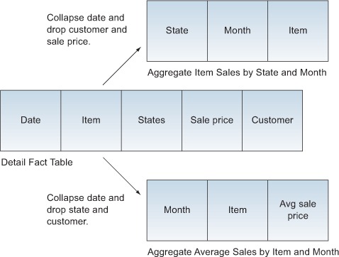
Aggregate tables aggregate data by collapsing and dropping dimensions. Collapsing a dimension means that the dimension is aggregated at a particular level, eliminating the finer-grained levels. In figure 7.5, the date dimension was collapsed to the month level, leaving off the days. If there were thousands of facts per day, this would reduce the size of the data by tens of thousands of rows.

Dropping a dimension means it’s left out of the aggregate table completely. You can think of this as the ultimate level of collapsing a dimension. A dropped dimension is essentially the same as the All Members level of the dimension. In figure 7.5, the aggregate average sales by item and month table dropped the customer and sale price columns because the only things we care about are identifying the items sold by state and month. In the average sales by item and month the customer and status were dropped to leave us with only the sales for each item by the given month.

7.3.1. Creating aggregate tables

The physical aggregate tables are created in the database and populated as part of the ETL process. There’s nothing special about the data in aggregate tables for Mondrian. Mondrian simply uses the data in the aggregate table when it has been configured to do so and the query can be answered by the aggregate table. It’s up to the ETL creator and database designer to properly populate the aggregate table.

Enabling aggregate tables

Aggregate tables can be enabled or disabled in the mondrian.properties file. For Pentaho they’re disabled by default. To enable aggregates, simply set the mondrian.rolap.aggregates.Use and mondrian.rolap.aggregates.Read properties to true.

There are a couple of different approaches that can be used to populate the aggregate table. The first, and most obvious, is to populate the aggregate table as the detailed fact table is being populated. But since the data needed for the aggregate table is in the detailed fact table, it’s recommended that you first populate the detailed fact table from the operational or staging data, and then populate the aggregate table from the detailed fact table. This has the secondary advantage that the fact and aggregate tables will be internally consistent. It also removes some of the logic common to populating facts, such as identifying new or modified facts.

Aggregation designer

Mondrian includes a tool called Aggregation Designer that can aid in creating summary tables. Aggregation Designer will read a schema and make recommendations for aggregate tables. It’ll then generate SQL that can create and populate the aggregate tables for you. You may still need to tweak the results, but this can save time when you’re getting started. Due to space limitations, we won’t cover Aggregation Designer in this book in detail. The tool and its documentation are available from the Mondrian site.

7.3.2. Declaring an aggregate table

Aggregate tables are declared as a special usage of the MeasureGroup tag first introduced in chapter 4. Listing 7.1 shows the declaration of an aggregate table for item sales by month. The first thing that makes this an aggregate table is the type='aggregation' attribute in the MeasureGroup element.

Listing 7.1. Declaring an aggregation table

Once the table is declared, a standard measure group is added. In this case, the aggregation includes all of the sales for a given item in a given month. Notice, however, that because this is a measure group, you can also introduce new measures that don’t exist in the original fact table. In this case, we’re introducing a new measure called [Average Sales], which is the average for all sales for the month for the item.

Now that the measures are defined, it’s time to declare the links. The first declaration, for the item, is the same declaration that you’d use in the detailed fact table using the ForeignKeyLink element. The next link, CopyLink, is a special element that specifies using that we’re copying a dimension with levels, but only down to the Month level in this case.

Aggregate tables in older versions of Mondrian

If you’re familiar with versions of Mondrian prior to version 4, you’ll notice that Mondrian no longer uses the AggName approach to creating aggregates. Mondrian has also made aggregate tables explicit and has dropped the pattern-matching approach to aggregate tables.

7.3.3. Which aggregates should you create?

The preceding simple example shows that many different types of aggregate tables can be created. If you have a large fact table with many dimensions and facts, you could create hundreds or thousands of aggregate tables. So how should you decide which aggregate tables to create?

It’s tempting to create as many aggregate tables as possible, but this is not recommended for several reasons. For one, the ETL process will grow as more aggregate tables are created and need to be populated. One of the reasons for using a ROLAP tool is to shorten the time needed to move data from OLTP systems to OLAP. Aggregate tables are a step in the direction of “pure” OLAP where intersections are precalculated, sometimes taking hours before data is available for analysis.

Aggregate tables also take up space in the analytics database and possibly in backups of the database. The additional storage in backups can be avoided by just storing the detailed facts and re-creating the fact tables, but this slows down the restoration process as well as makes it more complex.

Because it’s undesirable to create all the possible aggregates, careful performance testing can help you determine which ones will be most useful. If you have a good performance test environment and you know the common queries, you can find out which queries could use some performance help. Start with the queries, create an aggregate, and see what impact that has on performance. There are two nice benefits to this approach. First, it’s fairly easy to create and populate aggregate tables. Second, aggregates can be added after the fact to speed up slow queries, so it’s not essential to create all the aggregates you might eventually want the first time around.

Now let’s turn to Mondrian’s second significant performance tuning feature: caching. Whereas aggregate tables reduce the amount of data read from the database, caching can eliminate reads entirely by storing data in RAM. Because even the fastest read from the disk or the network is going to be thousands of times slower than in-memory reads, this can lead to another order-of-magnitude gain in performance.

7.4. Caching

The process of retrieving schemas, dimension members, and facts and then performing calculations can be costly from an I/O perspective. Even with column-based analytics databases and fast storage, such as solid state drives, disk I/O is still orders of magnitude slower than reading from memory. To speed up analysis, Mondrian can cache the data in memory and use that rather than going to the database for each call.

In this section we’ll first take a look at the different types of Mondrian caches, and then we’ll study the special case of the external segment cache.

7.4.1. Types of caches

Mondrian has three different caches, as shown in figure 7.6.

• The schema cache keeps schemas in memory so they don’t have to be reread every time a cube is loaded.
• The member cache stores member values from dimensions in memory, which reduces the number of reads from the database.
• The segment cache stores previously calculated values in memory so they don’t need to be retrieved or recalculated. This can significantly speed up analysis by reducing the number of reads for common calculations.

Figure 7.6. The different Mondrian caches

As of Mondrian 3.3, you can use external segment caching. External segment caches store segments in an optional data grid. In section 7.4.2 you’ll learn how to configure the external cache using several different technologies and when to use each.

All of the caches work together to maximize Mondrian performance, and the next few sections describe how they work. Understanding the caches is important for understanding when the caches should be primed or cleared.

Schema cache

The schema cache stores the schema in memory after it has been read the first time, and it will be kept in memory until the cache is cleared. This means that whenever you update the schema, you need to clear the schema cache. If you’re using Pentaho as your container, you can clear the schema cache by selecting Tools > Refresh Mondrian Schema Cache. Sometimes clearing all of the caches is required because Mondrian uses a checksum of the schema XML as the key for the cache. This becomes important if you have dynamic schema processors (discussed in chapter 9) because the dynamically generated schemas will be different. Attempting to clear just one schema will not clear all of them.

Member cache

The member cache stores members of dimensions in memory. As with the schema cache, there’s not much to worry about as far as configuring the member cache. Just keep in mind that as with the schema cache, the member cache can also get out of synch with the underlying data. Mondrian has a Service Provider Interface (SPI) that allows you to flush the members of the cache, as described in section 7.6.

The member cache is populated when members of a dimension are first read, and the members are retrieved as needed. If the member is in memory, it doesn’t need to be reread from the database, increasing performance.

Members, in this case, are specific values for levels in a dimension, such as [Time].[2011].[February] or [Customer].[All Customers].[USA].[WA], and they include the root and the children. It’s important to remember that a member is more than just a value, such as WA, but rather a value within a dimension level. This is because a member can have the same name for a given level, such as Springfield, for different paths within the hierarchy: [NA].[USA].[Illinois].[Springfield] versus [NA].[USA].[South Dakota].[Springfield].

Segment caching

The segment cache is probably the hardest to understand, but it’s also the cache that can have the biggest impact on performance. The segment cache holds data from the fact table, usually the largest table by an order of magnitude or so, and it has aggregated data. Holding data from the largest table can dramatically reduce the amount of I/O that takes place, and caching aggregated data reduces the number of calculations that need to occur.

Listing 7.2 shows the conceptual structure of a segment. First, the segment deals with a particular measure, in this case Internet Sales. Second, the segment contains a set of predicates, or member values, for which the data is relevant. In this case, the data is internet sales for males who graduated high school across all years. Finally, the segment carries the actual data values that make up the segment. If a request includes the predicates already stored, the data values can be quickly aggregated from the in-memory values rather than making a SQL call to the database.

Listing 7.2. Conceptual segment structure

Measure = [Internet Sales]
Predicates = {
  [Gender = Male],
  [Education Level = High School],
  [Year = All Years]
}
Data = [1224.50, 945.12, ...]

7.4.2. External segment cache

The external segment cache is a newer feature introduced in Mondrian 3.3. It’s an optional physical implementation of the segment cache described previously. Whereas the standard segment cache stores segments in local memory, the external segment cache stores data in a data grid. This allows you to extend the amount of data stored in memory by adding additional servers. In some cases, it also provides in-memory failover of the cache, as you’ll see in the next section. Although reading data across the network is substantially slower than reading from local memory, it’s typically still an order of magnitude faster than reading from the database and performing calculations.

Figure 7.7 shows the high-level architecture for the external segment cache. Mondrian creates aggregations of measures to return for the query, and each aggregation is made up of segments as described previously. The segment loader is responsible for loading the segments, and it’ll first attempt to retrieve the segment from the cache. If the segment isn’t stored in the cache, the segment loader will query the database and then put the segment in the cache. The segment is then returned to Mondrian to use as part of the resulting aggregation.

Figure 7.7. External segment cache architecture

There are currently three external segment caching technologies available for Mondrian. The first two, Infinispan and Memcached, are available as part of the Pentaho Enterprise Edition solution. The third, Community Distributed Cache (CDC), is available as an open source solution. There are tradeoffs to using each of the solutions. If you have an enterprise license for Pentaho, you’ll want to stick with Infinispan or Memcached, since those are the only ones supported. If you’re using Pentaho CE, then CDC is a good choice.

Note that there is technically another choice, the Pentaho Platform Delegating Cache, but at the time of writing, this cache was still experimental and not recommended for production use. Infinispan and Memcached should be used instead.

Your own data grid

An additional option that we won’t cover is that you can create your own data grid for external segment caching. To do so, you’d need to implement the mondrian.spi.SegmentCache interface and then configure Mondrian to use your solution. The three solutions covered in this chapter make the need for such an approach rare.

Installing the external cache plugin

The external segment cache isn’t automatically installed with Pentaho. To use the external cache with Pentaho EE, you need to get the analysis EE plugin, available to users of the Enterprise Edition of Pentaho. You’ll need to download the pentaho-analysis-ee plugin package from your software site. Fully up-to-date instructions can be found on Pentaho’s Infocenter at http://infocenter.pentaho.com/help/topic/analysis_guide/topic_cache_control.html. Using CDC with Pentaho CE is discussed later in this section.

The plugin consists of two parts. The first is a lib directory that includes all of the JAR files needed to support the plugin. These files get deployed as part of the running application. If you’re running inside of Pentaho’s BA server, then these are deployed to the lib directory of the app server. For Tomcat, this is the tomcat/webapps/penataho/WEB-INF/lib folder. If you’re running Mondrian standalone under Tomcat, this is the tomcat/webapps/mondrian/WEB-INF/lib folder. Other embedded uses of Mondrian need to have all of the files deployed so that they’re in the classpath.

Watch the version numbers!

All of the library files for Mondrian contain version numbers, such as jgroups-2.12.0.CR5.jar. This can cause problems if a different version of the same file already exists in the classpath. Be sure to replace such files if they exist.

The second directory, called config, contains all of the configuration files. These files all need to be copied to a location in the classpath as well. For Pentaho and Mondrian running under Tomcat, this is the WEB-INF/classes folder, and other servers will have a similar location. The important thing is that the files must be accessible to the Java classloader when the application is run.

Once everything is deployed, you need to configure Mondrian to use the external segment cache of your choice. The main configuration file is pentaho-analysis-config.xml, and its purpose is to turn external segment caching on or off and to specify the caching technology to use. To enable caching, set the USE_SEGMENT_CACHE entry to true. To specify the caching technology to use, set the entry for SEGMENT_CACHE_IMPL to have the name of the class that handles the cache. By default, Pentaho configures the Infinispan version as the recommended implementation, but the other caching technologies are also preconfigured and simply need to be uncommented. If you’re using any other approach, add an entry for the custom class.

Infinispan

Infinispan is an in-memory data grid that uses JGroups peer-to-peer communications to communicate between servers. Figure 7.8 shows the architecture when using Infinispan. Each server in the cluster has a copy of Infinispan running locally, and the servers share data across the network using peer-to-peer communications. In the case of Pentaho, the default is to use JGroups.

Figure 7.8. Using Infinispan for the external segment cache

Infinispan has a few features that make it an ideal default. Infinispan shares segments, which means that any node can store a segment in the cache and any other node can retrieve it. Infinispan also can be configured to have multiple copies of the segment in the cache. This allows a server to fail, and the segment to still be available to the cluster without rereading the data. Finally, Infinispan will attempt to store and retrieve data locally to minimize network traffic and latency. Because most segments will be relevant to the analysis currently being performed within a server, this makes the overall performance better.

Infinispan has one drawback: it has no standalone nodes. To scale Infinispan you have to add additional servers. Because many deployments of Mondrian run in a horizontally scaled environment (one with multiple servers in a cluster), this is not usually a problem. But if you’re not running in a cluster, Memcached may be a better choice.

Configuring Infinispan

You can configure Infinispan by modifying the infinispan-config.xml file. For full configuration instructions, you can refer to the Infinispan site: www.jboss.org/infinispan/. But you may just want to change the numOwners setting. This attribute specifies the number of different nodes that will have a copy of the data. The default is 2, but it can be set higher. The more copies, the safer the data is from loss due to server failure. The tradeoff is that the more copies you have, the slower the cluster becomes. Because the original segment is always persisted in the underlying database, a low number is recommended.

Infinispan comes preconfigured to work with JGroups, a peer-to-peer communication technology. You can change this configuration or replace it altogether. See the Infinispan documentation and JGroups documentation (www.jgroups.org) for details. One change you can easily make, however, is changing the communication protocol used by JGroups. Simply modify the value of the configurationFile property in the infinispan-config.xml file to use a different file. By default, UDP is configured, but you can also configure it to use TCP or EC2 if you’re deploying to Amazon’s EC2 cloud. The filenames are of the form jgroups-protocol.xml, where protocol is udp, tcp, or ec2.

Memcached

Memcached is an alternative to Infinispan, and it uses a different architecture, as shown in figure 7.9. Memcached is a master/server data grid that stores key/value pairs. Mondrian interacts with the master to store and retrieve segments from memory. The master node will then store the data in one of the server nodes with a key and a value.

Figure 7.9. Using Memcached for the external segment cache

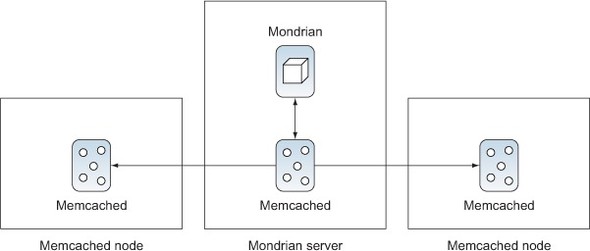
The major benefit that you get from Memcached is that it’s easy to add additional memory nodes. Simply create a server with memory, and install and run Memcached. Then configure the master node to use the additional server. This differs from Infinispan, which requires a much heavier-weight server. Memcached is ideal for vertical scaling where a large, fast server is used to support fewer users but lots of data.

The major drawback to Memcached is that there is no sharing or failover. If multiple servers are using the same Memcached servers, the segments won’t be shared between nodes. If the master node goes down, the cache is essentially lost from memory, although it can be reread from the database.

Configuring Memcached

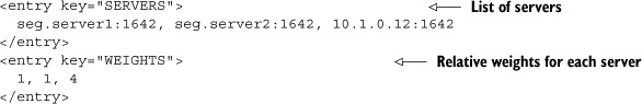
Configuration for Memcached is done using the memcached-config.xml file. This file has a number of configuration values, most of which can be left at their default values. But there are two that you’ll need to modify: SERVERS and WEIGHTS.

The SERVERS setting contains a comma-separated list of all of the server and port addresses of running Memcached servers. To add another server, simply add the IP address or DNS name plus port number that the Memcached server is listening on.

The WEIGHTS setting is a comma-separated list of integers that describe the relative amount of memory for each server, in the same order as for the SERVERS setting. For example, suppose that you have three servers: the first two have 1 GB of RAM and the third has 4 GB of RAM. The WEIGHTS setting would contain 1, 1, 4, indicating that the fourth server has four times as much RAM available. The weights are relative, so 2, 2, 8 would work just as well. You should try to anticipate the smallest server setting and make that value 1, with all other values being multiples, although you can always change it in the future by reconfiguring. Listing 7.3 shows a snippet of a configuration file with three servers.

Listing 7.3. SERVERS and WEIGHTS configuration example

Community Distributed Cache (CDC)

CDC is an open source alternative to Infinispan or Memcached from Webdetails (http://cdc.webdetails.org) based on Hazelcast. Its architecture, shown in figure 7.10, is similar to Memcached in that it can support standalone memory nodes. But CDC has additional features that are not standard when using either Infinispan or Memcached.

Figure 7.10. Community Distributed Caching architecture

In addition to caching for Mondrian, CDC provides caching for Community Data Access (CDA), a multisource data abstraction that we’ll discuss more in chapter 9. As a Pentaho plugin, CDC provides administration tools that let you see the state of the caching directly in the user console. It also enables you to clear the Mondrian cache, which normally requires writing software.

The easiest way to install CDC is to use the CTools Installer that’s available for download from https://github.com/pmalves/ctools-installer. Once you’ve downloaded the installer, run it as an administrator with the following command: ctools-installer.sh -s solutionPath -w pentahoWebapPath -y. The solutionPath is the absolute path to your pentaho-solutions directory, and pentahoWebapPath is the directory for the Pentaho web application, such as /.../tomcat/webapps/pentaho. This latter setting is optional in the script, but it must be specified for CDC to be installed.

wget required

The CTools Installer script uses wget, a common tool for downloading content from the web. wget is not automatically installed on all platforms, particularly Windows and more recent versions of OS X. Download and install wget (http://ftp.gnu.org/gnu/wget) before attempting to install CDC.

Once you have CDC installed, you’ll want to install one or more standalone servers for caching. The standalone node can be downloaded from http://ci.analytical-labs.com/job/Webdetails-CDC/lastSuccessfulBuild/artifact/dist/cdc-redist-SNAPSHOT.zip. Simply use the launch script appropriate for your operating system to start Hazelcast. The nodes will find one another, so no additional configuration is required. You’ll see messages similar to the following in the terminal window showing the known Hazelcast servers.

Listing 7.4. Hazelcast server showing two servers

Members [2] {
                 Member [10.0.1.7]:5701 lite
                 Member [10.0.1.7]:5703 this
             }

Once CDC and related tools are installed, you need to tell Pentaho to start using CDC for caching. Simply log into the Pentaho User Console and select the CDC icon in the toolbar. Eventually CDC will load and give you an option to start caching (see figure 7.11).

Figure 7.11. Community Distributed Caching configuration

After toggling or otherwise changing the configuration of CDC, you must restart the Pentaho application server. Once you do, if you use a tool that uses Mondrian you’ll see the cache start to fill. CDC provides a simple console that displays information about the cache and memory usage under the Cluster Info tab (see figure 7.12).

Figure 7.12. CDC cluster summary

Setting Saiku to use the same Mondrian as the BI Server

By default, Saiku is deployed with its own Mondrian version and files. In this section, we configured CDC to work with Mondrian on the BI Server, so Saiku will not be able to take advantage of CDC clustering. You can change this by running the saiku-shareMondrian.sh script located in the pentaho-solutions/system/saiku folder and providing the path to the Pentaho web app, usually tomcat/webapps/pentaho.

7.5. Priming the cache

Mondrian will automatically update the caches as schemas and dimensions are read and aggregates are calculated. This means, however, that the first user to access the data is populating the cache rather than getting the benefits of it. What you really want is the ability to prepopulate the cache before business users start performing analysis. Because the cache is populated as part of returning the results of a query, this means any call that makes a query to Mondrian will populate the cache.

The first question you need to ask is which queries need to be run. One approach is to simply wait for users to complain about slow reports, but a much more proactive approach is available. Simply turn on the Mondrian MDX log and monitor it for queries that take a long time. Long is relative, but if there are queries that take more than a minute or so, they are good candidates for precaching.

There are a number of approaches available for precaching that can be used. All reports in Pentaho are URL-addressable, so all slow reports can be called from a script, populating the cache. Another approach, when using Pentaho, is to create an action sequence that makes calls to Mondrian, populating the cache. Probably the simplest approach, though, and one that works with most Mondrian installations, is to use XML for Analysis (XMLA) web service calls.

XMLA is a SOAP-based standard for making web service calls. All you need to do for this to work is to expose Mondrian cubes as XMLA data sources. By default, when cubes, called catalogs in XMLA, are deployed to Pentaho, they’re also made available as XMLA data sources. Other configurations, such as running Mondrian standalone, also support XMLA.

Chapter 10 will give more specifics on XMLA, so we won’t cover it in detail here. What we will do here is create a web page that will make calls to XMLA using Ajax. We’ll handle the responses, but only to note whether the call was successful or not. This web page could then be called whenever the cache needed to be populated.

Cross-domain considerations

As a security constraint, JavaScript won’t allow calls to other domains. That means a script running on mydomain.com can’t call a web service on yourdomain.com. There are ways to get around this constraint, but in this case the cache refresh page can simply be deployed to the same server, because it adds minimal overhead.

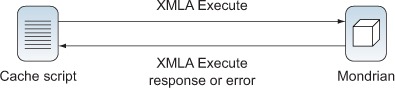
Figure 7.13 shows the sequence of messages that our script will handle. The script will send a series of XMLA Execute messages (discussed in chapter 10) to the Mondrian server. The server will then respond with either an error message if there was an error, or a response to the XMLA query. The script will accept responses and log the errors and results to the web page. If MDX logging is enabled, you can also view the logs to see what queries were run.

Figure 7.13. Performance analysis process

The details of sending XMLA messages are covered in detail in chapter 10, so we’ll just focus on the specifics for enabling caching. To make the script reusable and extensible, we’ve created a separate script that has the catalogs and queries to execute. Listing 7.5 shows the configuration and queries to be made, as well as the connection info.

Listing 7.5. MDX queries

The connection information is simply the location of the server and the user information for login. The DatasourceInfo is specific to the installation, but it’s otherwise static; this example shows the data source info for Pentaho. Other ways of running Mondrian will have a similar data source.

The final part of the file identifies the catalogs (schemas) and queries that will be run by the script. The catalogs are organized in an array with each containing an array of queries. This makes it easy to add additional catalogs and queries to be run. Simply update this one JavaScript file and rerun the script.

Shared caches

In this example, we have a single user, joe, that we are using to prime the cache. Only schemas and data that joe has permissions to see will be put into the cache. This may mean that you need to run multiple versions of the queries with different users to prime all the caches.

Listing 7.6 shows the simple page that runs the script. In addition to including the needed scripts and style sheet, it has two <div> sections called results and errors. The script will write the results and errors to these sections when the page is run.

Listing 7.6. XMLA cache web page

<html>
  <head>
    <title>XMLA Cache</title>
    <link rel="stylesheet" type="text/css" href="XMLACache.css" />
    <script src="jquery-1.7.2.js"></script>
    <script src="MDXQueries.js"></script>
    <script src="XMLACache.js"></script>
  </head>
  <body>
    <h1>Pre-Cache Mondrian via XMLA</h1>
    <div id="results"></div>
    <div id="errors"></div>
  </body>
</html>

Listing 7.7 shows the main loop of code that runs the queries. When the main HTML document is ready, the script simply iterates over the catalogs and queries, making an XMLA call for each query.

Listing 7.7. Execute MDX queries

$(document).ready(function() {

  $("#results").html("<h2>Results</h2>");
  $("#errors").html("<h2>Errors</h2>");

  for (var idx = 0; idx < queries.length; idx++) {
    catalog = queries[idx];

    for (var qidx = 0; qidx < catalog.queries.length; qidx++) {
      postMessage(
        getQueryMessage(catalog.queries[qidx],
                        dataSourceInfo, catalog.catalog),
        'xml', handleQueryCallback);
    }
  }

});

Figure 7.14 shows the results of executing the query. In this case, two of the queries were successful and one failed. Examining the error message as well as the Mondrian logs will tell you which queries failed. At this point, the caches have been prepopulated with data from the successful queries and are ready for use.

Figure 7.14. XMLA cache results

Now that you know how to prime the caches, the next consideration is how to clear them. You need to do this whenever the underlying data has changed, making the caches out of date. The next section shows how to programmatically clear each of the caches.

7.6. Flushing the cache

The drawback to caching is that while the data is stored in memory, the original data source can change, putting the cache out of sync with the true data. This usually occurs when ETL is performed. This section discusses ways to flush the cache, including using the console (for the schema cache) as well as the Cache Control API.

7.6.1. Flushing the schema cache

The schema cache keeps each of the unique caches in memory. The key for each cache is a checksum for the schema. When the schema is flushed from the cache, its associated member and segment caches are flushed as well, making this a brute-force approach. But if the schema has changed, or if determining the details of what to flush is too complex, this can be the best approach and certainly is the simplest. The caches can be repopulated using the techniques described in the previous section.

Most tools using Mondrian, such as Pentaho, provide a way to manually flush the cache. In Pentaho you can use the Enterprise Console or User Console. If you’re logged into the User Console as an administrator, simply select Tools > Refresh > Mondrian Schema Cache.

The manual approach works fine, but administrators usually want to automate cache flushing as part of the overall ETL workflow. Figure 7.15 shows how Mondrian and the cache fit into the overall ETL workflow. After populating the OLAP database, Mondrian is called to flush and then prime the cache. This process makes sure the cache is synchronized with the underlying database so that when analysis is performed, the data is up to date.

Figure 7.15. Caching and the ETL workflow

To make it easy to integrate flushing the cache into the ETL process, you can create a class that contains methods to flush parts of the cache. You can also create a JSP that uses the new class. It then becomes easy to flush the cache by calling a URL with the appropriate parameters.

Table 7.1 shows the three scenarios that the flushing tool will support. The scenarios run from flushing everything to flushing a specific region of the cache. Mondrian’s cache control SPI is very detailed and can allow you to control any parts of the cache, so these are only examples of what’s possible.

Table 7.1. Cache-flushing scenarios

What to flush	Parameters required
Everything	No parameters
Specific cube	Catalog and cube
Specific region	Catalog, cube, and members

Listing 7.8 shows some JSP code that controls caching. It receives parameters and then calls to the CacheFlusher class to flush the appropriate parts of the cache. This makes it easy to separate the work of flushing the cache from the user interface. The same class could be used in an action sequence or be embedded in an application if appropriate.

Listing 7.8. JSP to flush the cache

To flush the entire cache, you can simply call the JSP with no parameters. For example, if the JSP is deployed to the public folder of the Pentaho web app on the local machine, you’d call http://localhost/pentaho/public/FlushCache.jsp. This would invoke the flushAll() method of the CacheFlusher class, shown in listing 7.9. Note that this will only apply to new connections. Existing connections will continue to use the previous information.

Listing 7.9. Flush the entire schema cache

Flushing everything when only some data has changed is excessive and will decrease performance unnecessarily for other cubes unless everything is primed again. If only the data for one cube has changed, then only that cube’s cache should be flushed. The next section will show how to flush a single cube’s cache at a time.

7.6.2. Flushing specific cubes

In an environment where there are many different schemas and cubes, there may be multiple ETL processes that only apply to a specific cube. After the data has been updated, then only the caches for the cubes that have been impacted need to be changed. This means that other cubes will continue to use the cache. As with clearing everything, this will only affect new connections.

Listing 7.10 shows the code to clear a specific cube’s cache. To clear the cache, simply call the JSP and specify the catalog and cube to clear.

Listing 7.10. Flush a single cube’s cache

This will work fine if you want to clear the cache for the entire cube. But often only parts of the cube will be updated, particularly when time is a dimension, because past facts shouldn’t change. The next section describes how to flush specific regions of the cube’s cache.

7.6.3. Flushing specific regions of the cache

Flushing specific regions of the cube’s cache gives the finest control over the cache. Suppose that Adventure Works has been tracking sales for several years. They also have a nightly batch process that updates the data warehouse from the operations database. They would only need to clear the cache for any information that has changed, such as the sales for the current month.

Listing 7.11 shows the code needed to flush a region. It looks a bit complex, but it actually only has a few key calls you need to understand. The code for finding the schema and cube should look familiar by now, so we’ll only focus on the code for clearing the regions.

Listing 7.11. Flush the region of a cube

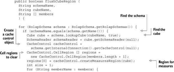
The cell regions are a set of cells in the cube that need to be cleared. There’s always the measure region, so that gets added as the first region to include. Then each member passed in gets converted to a cell region as well. The memberNameToSegmentList method converts from the member name to a special list of members.

Once all of the regions are defined, a cross-join is created and the cache control object flushes the region. The next call to Mondrian that needs the cells in the specific region would read them from the database and populate the cache. If this could be a lot of data, the cache-priming techniques discussed earlier could be used.

7.7. Summary

This chapter covered a number of topics related to improving the performance of very large Mondrian installations. One or more of these approaches can be used, and each provides a different advantage. These are the key points to remember:

• Performance is something to consider up front and plan for.
• Performance tuning is an iterative process.
• A finely tuned database is the first step to high performance.
• Mondrian uses multiple caches to improve performance, including schema, member, segment, and external segment caches.

Now that you have a grasp on Mondrian performance tuning, it’s time to return to data security. The next chapter will show you how to dynamically apply security based on user information.