
Chapter 11. Advanced analytics
This chapter is recommended for
| Business analysts | |
| Data architects | |
| Enterprise architects | |
| Application developers |
In this chapter we’ll cover how to do more advanced analytics both inside Mondrian and with external tools. The advanced analytics inside Mondrian, through MDX, meet many use cases. Adventure Works will find many of their common analytics, metrics, and scorecards can be built using these. You can run the MDX examples we present in this chapter; we cover the MDX in more detail than external tools. We’ll also explore some limited “What If” support to allow Mondrian to help you model and think about various scenarios. We’ll then delve into the external tools and briefly cover where Mondrian fits within the Big Data landscape and what tools are often used with Mondrian for data mining. These topics are primarily aimed at the business analyst and enterprise architect.
11.1. Advanced analytics in Mondrian with MDX
Mondrian’s query language, MDX, provides a variety of advanced time-based analytics that you can leverage immediately on top of your existing cubes. MDX supports (and makes rather easy) things like “year to date” accumulations, this quarter versus the same quarter last year, percent increase of this quarter over last quarter, and on and on. We’ll explore and build some of these calculations in this section.
MDX stands for Multidimensional Expressions; it was made popular by Microsoft as part of their SQL Server Analysis Services. Until 2000, no consistent vendor-agnostic way to query OLAP cubes existed. Unlike relational databases that had a similar SQL dialect between vendors, OLAP systems all had individual and disparate APIs. At about the same time, Microsoft’s dominance and market leadership in the OLAP server space made MDX a de facto standard, since the majority of the market (already SQL Server) already knew MDX. Made official, as part of a multi vendor standard (XML for Analysis), MDX has become the only well-implemented query language for OLAP systems. Mondrian, like many other OLAP systems, chose it for its compatibility and eloquence.
Calculations in MDX are powerful, not necessarily because of their raw function. For instance, knowing that you can do arithmetic such as (A - B) in a language isn’t that impressive. What’s impressive about MDX is that every calculation is aggregation-and level-aware. What does that mean? Our simple calculation (A - B) need not explicitly say at which level of aggregation it applies. For Adventure Works, this means they can define (A - B) in MDX and it works if A and B are calculated at the [Year] level, [Month] level, [All Products] level, [Product Category] level, and so on. Calculations are inherently and magically useful all over the cube at different levels of aggregation. In fact, unless you deliberately make your MDX use a specific level ([Country]), it’ll apply to all levels. Contrast that to SQL, which requires the level of aggregation (aka the GROUP BY clause) to be defined in the query with the calculation. In MDX, the calculation is defined and MDX makes sure the calculation is done on the proper level of aggregation.
MDX is a big topic; there are entire books on writing MDX, and we’ve linked to resources devoted to the query structure and basics in appendix B. Here we hope to give you the basics to be able to run, see the results from, and have a quick list of common MDX calculations you can use on your Mondrian project.
One time versus saved in cube
Often, fancy MDX fragments are developed using a free-form MDX query tool (such as the query box in Saiku). Once developed, and useful, it’s best to take the new calculation (This Quarter versus Same Quarter Last Year) and make it a calculated member. This allows anyone using the cube in Saiku or Analyzer to use the powerful calculation, without needing to know anything about MDX (refer back to section 5.4.2 for details).
This saving of MDX fragments into the cube is the Mondrian equivalent of a database view. It’s a prebuilt set of logic ready to execute, but for the user it appears as a simple “thing” to get data from.
11.1.1. Running MDX queries
In this section, we’ll make sure you know how to run MDX queries and see the results using the sample platform. We’ll also show you the WITH MEMBER syntax.
First, in order to run the MDX fragments in this section, you’ll need to use Saiku. Using the sample virtual machine provided for the book, you’ll need to make sure that Pentaho is running. Once it is, to launch Saiku you’ll want to log in to the User Console, and then click the File menu, then New, then Saiku Analysis. Once you see Saiku, you’ll want to select the FoodMart Schema/Sales Cube from the drop-down list. Once you’ve done that, you should see Saiku ready to help you drag and drop to create a query. But we’re going to use the MDX editor to manually write our MDX instead.
There’s a button on the toolbar titled Switch to MDX Mode. You’ll want to click this button, and then you should see a free-form text box that will allow you to enter the MDX examples in this chapter. You can copy and paste (if you have the eBook) directly into the text box, then click the Green arrow to run the query.
We’ll make extensive use of the WITH MEMBER MDX syntax. This MDX construct allows us to create calculations that exist only in the single query. Earlier in this chapter we covered how to make those changes more permanent.
Now that you know how to run MDX queries and see the results, let’s get on to specific formulas that you’ll hopefully find useful.
11.1.2. Ratios and growth
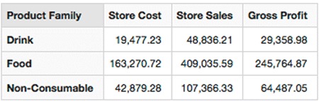
We’ll start with a straightforward post aggregation calculation using arithmetic. Say Adventure Works would like to calculate [Gross Profit]. Its calculation is straightforward: [Store Sales] - [Store Cost]. We can make this calculation simply in MDX (listing 11.1 and displayed in figure 11.1).
Figure 11.1. [Gross Profit] results
Listing 11.1. [Gross Profit] MDX

The results in figure 11.1 demonstrate simple subtraction; it’s worth noting that this calculation is happening in memory in Mondrian after the main aggregation and [Store Sales] and [Store Cost] is calculated in the database. Remember, as we mentioned previously in this section, this calculation is aggregation-safe so it’ll work the same if it’s at the [Product Family] level, or one level below at the [Product Department] level. For instance, here is the exact same calculation working at the [Product Department] level; note that the WITH MEMBER fragment is identical (listing 11.2 and figure 11.2)!
Figure 11.2. [Gross Profit] at [Product Department] level

Listing 11.2. [Gross Profit] at [Product Department] level
WITH MEMBER [Measures].[Gross Profit] as
' [Measures].[Store Sales]
   - [Measures].[Store Cost]'

SELECT
{[Measures].[Store Cost]
, [Measures].[Store Sales]
, [Measures].[Gross Profit]} ON COLUMNS,
{[Product].[Product Department].Members} ON ROWS
FROM [Sales]
The simple arithmetic in MDX also allows us to create important ratios and proportions. For Adventure Works, the overall gross profit percentage (the [Gross Profit] as a proportion of the [Store Sales]) is also salient. Without these types of proportions and percentages, it would be hard to gauge relative effectiveness when comparing scalar values of different magnitudes. For instance, looking at the raw [Gross Profit] for individual [Product Family]s might not help you figure out which [Product Family]s are contributing to Profit effectively (as a percentage) if you’re looking at raw numbers. As we see in figure 11.3 the [Product Family]s have orders of magnitude difference [Gross Profit]; you have to look at the ratio to determine the relative profitability of each [Product Family].
Figure 11.3. [Gross Profit Margin]

Listing 11.3. [Gross Profit Margin] MDX
WITH MEMBER [Measures].[Gross Profit] as
' [Measures].[Store Sales]
   - [Measures].[Store Cost]'
MEMBER [Measures].[Gross Profit Margin] as
'[Measures].[Gross Profit] / [Measures].[Store Sales]'

SELECT
{[Measures].[Gross Profit]
 ,[Measures].[Gross Profit Margin]} ON COLUMNS,
{[Product].[Product Family].Members} ON ROWS
FROM [Sales]
Note in figure 11.3 that the [Gross Profit] is wildly different for different [Product Family]s but the [Gross Profit Margin] is identical. Drinks, Food, and Non-Consumables all have a gross margin of 60%.
The last piece we’ll cover, in terms of cool arithmetic in MDX, is the ability to also create ratios and proportions at different levels. For instance, say we want to see what a particular [Customer].[State]’s contribution is toward the [Store Sales] for the [Country]. We can use the simple MDX arithmetic along with MDX’s ability to navigate levels in a hierarchy to display this data. We’ll use two MDX constructs. First, we’ll find our current member (Seattle, WA, or CA) in the hierarchy that’s currently being evaluated for calculation. The syntax for this is [Customer Geography].CurrentMember. Next, we’ll use the ability of any member to navigate to other places in the hierarchy. We’ll do this using the [Member].Parent function that gets the parent of any member ([USA] is the parent of [WA]). We’ll explore both CurrentMember and Parent in listing 11.4; we’ll divide each member’s sales by its parent’s sales—[State]’s total divided by the [Country] total.
Listing 11.4. [Sales % of Geography] MDX
WITH
MEMBER [Measures].[Sales % of Geography] as
'([Customers].CurrentMember, [Measures].[Store Sales])
/([Customers].CurrentMember.Parent, [Measures].[Store Sales])'

SELECT
{[Measures].[Store Sales]
 , [Measures].[Sales % of Geography]} ON COLUMNS,
NON EMPTY Hierarchize(
{[Customers].[State Province].Members,[Customers].[Country].Members
}) ON ROWS
FROM [Sales]
In figures 11.4 and 11.5 we can see the results of expressing the [Member].Parent as a percentage. OR represents approximately 25% of USA’s profit.
Figure 11.4. Sales percentage of total table
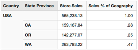
Figure 11.5. Sales percentage of total chart

Level-agnostic calculations
Remember, as long as you don’t pick a specific level, such as [Customer Geography].[State] in your MDX statements, and you use CurrentMember and the general CurrentMember.Parent for these types of calculations, they’ll work “up and down” the hierarchy. The same calculation, [Measures].[Sales % of Geography], can be used for City to State, State to Country, and Country to All Geographies.
11.1.3. Time-specific MDX
Prior Period is useful when you’re trying to calculate the classic month-over-month growth. Adventure Works has built this month-to-month growth report many times in SQL and knows their users will need to see it regularly! Using the MDX Member function .PrevMember you can positionally go back one day, month, quarter, or year. The .PrevMember is level-agnostic, so the same calculation can be used for any level in the hierarchy. We’ve also built on these raw growth figures and added some simple ratios using the arithmetic MDX we covered in section 11.1.2 to give an idea of the total velocity of the data. Adventure Works knows that although the raw growth values are interesting, their users want to see it as a percentage, ideally.
Listing 11.5. [Prior Sales] MDX
WITH
MEMBER [Measures].[Prior Sales] as
'([Time].CurrentMember.PrevMember, [Measures].[Unit Sales])'
MEMBER [Measures].[Prior Sales Growth] as
'[Measures].[Unit Sales] - [Measures].[Prior Sales]'
MEMBER [Measures].[Growth %] as
'[Measures].[Prior Sales Growth] / [Measures].[Prior Sales]'
,FORMAT_STRING='0%'

SELECT
{[Measures].[Unit Sales]
 ,[Measures].[Prior Sales]
 ,[Measures].[Prior Sales Growth]
 ,[Measures].[Growth %]
} ON COLUMNS,
NON EMPTY {[Time].[Month].Members} ON ROWS
from [Sales]
In figures 11.6 and 11.7, we can see, on a month-by-month basis, the growth (as a percentage) of sales over the previous month’s sales. Once again, we’ve used the scalar figure (such as -671 for Month 2) and arithmetic to arrive at the percentage which is preferred.
Figure 11.6. [Prior Sales] results

Figure 11.7. Prior Period chart

Adventure Works also knows that it’s common for their users to need to calculate the aggregated year-to-date totals for a variety of measures. They know this cumulative type aggregation is useful and often requested from their users. The MDX YTD() shortcut function (see listing 11.6) returns all periods from the beginning of the year right up to the current period and aggregates the totals to give the total year-to-date value. Figures 11.8 and 11.9 show the results.
Figure 11.8. [YTD Sales] results
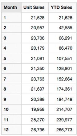
Figure 11.9. Year-to-date chart

Listing 11.6. [YTD Sales] MDX
WITH
MEMBER [Measures].[YTD Sales] as
'Aggregate(YTD([Time].CurrentMember), [Measures].[Unit Sales])'

SELECT
{[Measures].[Unit Sales]
 ,[Measures].[YTD Sales]
} ON COLUMNS,
NON EMPTY {[Time].[Month].Members} ON ROWS
from [Sales]
We’ve seen how Adventure Works can use YTD(), which returns the periods up to this point in the year and then use the generic Aggregate() MDX function to total those periods. The Aggregate MDX function will use the basic aggregator for the measure (Count, Sum, and so forth).
11.1.4. Advanced MDX
It’s common to develop some sort of target to base your current results against. Adventure Works sometimes has fixed targets (145,000 in sales per quarter), and other times they’re calculated from past performance. Though listing 11.7 shows a fixed target, it’d be just as easy to find the previous quarter’s figures, add 5%, and make that the “target.” Just like many of the other raw figures, we also adorn it with some percentages to make the real metric and velocity of the figures easily apparent to Adventure Works users.
Listing 11.7. Fixed-goal MDX
WITH
MEMBER [Measures].[Sales Goal] as
'145000'
MEMBER [Measures].[% from Goal] as
'([Measures].[Sales Goal] - [Measures].[Store Sales])
  / [Measures].[Sales Goal]',FORMAT_STRING='0%'

SELECT
{[Measures].[Store Sales]
,[Measures].[Sales Goal]
,[Measures].[% from Goal]
} ON COLUMNS,
NON EMPTY {[Time].[1997].Children} ON ROWS
from [Sales]
Note in figures 11.10 and 11.11 that the deviation from the goal, as a percentage, is readily apparent in the line chart.
Figure 11.10. Fixed-goal table

Figure 11.11. Fixed-goal chart

Adventure Works knows their users will want to see “What’s the overall trend?” If we continue on this general sales pattern, ignoring the natural noise of the month-to-month data, what will our sales be like in three months? Performing a linear regression (with the LinRegPoint() MDX function) allows Adventure Works to show the overall trend over a period of time. This avoids anxious calls from analysts who are worried about a single-month drop-off; linear regressions help to smooth out data and make general, unsophisticated forecasts for the future. We’ll discuss the ability to employ more sophisticated forecasting options later in section 11.3.
Listing 11.8. Trend-line MDX
WITH
MEMBER [Measures].[Sales Trend] as
'LinRegPoint(
  Rank(
     [Time].CurrentMember,
     [Time].CurrentMember.Level.Members),
  {[Time].CurrentMember.Level.Members},
   [Measures].[Unit Sales],
   Rank(
       [Time].CurrentMember,
       [Time].CurrentMember.Level.Members)
)'


SELECT
{
[Measures].[Unit Sales]
,[Measures].[Sales Trend]
} ON COLUMNS,
NON EMPTY {
[Time].[Month].Members} ON ROWS
from [Sales]
Note in figures 11.12 and 11.13 that a general trend for sales over the past 12 months is now projecting out into the future where we don’t have sales figures. LinRegPoint() gives Adventure Works the ability to do simple forecasting on any measure.
Figure 11.12. Trend-line table

Figure 11.13. Trend-line chart

Adventure Works also needs to explore “What are the best months for sales in the past 12 months?” In listing 11.9 we explore how to discover the 10 best months across the entire company. Ranking (via the MDX Rank() function) allows you to order and rank results and determine sets of performers. Figure 11.14 shows the output for Adventure Works.
Figure 11.14. Ranking table

Listing 11.9. Ranking in MDX
WITH
MEMBER [Measures].[Sales Rank] as
' Rank(
     [Time].CurrentMember

     ,[Time].CurrentMember.Level.Members
     ,[Measures].[Store Sales])'

SELECT
{
[Measures].[Store Sales]
,[Measures].[Sales Rank]
} ON COLUMNS,
NON EMPTY {
Head(
 Order([Time].[Month].Members, [Measures].[Sales Rank], BASC)
 , 10)
} ON ROWS
from [Sales]
In listing 11.9 we saw how to get the relative, ordinal rank of a figure among its peers. We also tacked on the use of two additional MDX functions that are commonly used with this type of analysis. Order() changes the order of members based on a value. In listing 11.9 we ordered by the Rank() we just created. Next we used Head() to only grab the first 10 items in the list of all ranked months.
Now that we’ve covered some of the advanced analytics we can accomplish using Mondrian by itself, with MDX we move on to more advanced analytics. Next we discuss what happens when we want to play around and make changes to data values for what-if analysis.
11.2. What-if analysis
Mondrian has some support for helping you explore some “What If” analysis. Most reporting systems present the user with data as it is; static data provides little if any help for the data analyst’s desire to explore scenarios that haven’t actually happened. In fact, Mondrian’s term for such what-if analysis is scenarios.
Scenarios allow users to make nonpermanent changes to values in the cube for the purpose of seeing how those changes affect totals, other ratios, and other metrics. Take for instance a hypothetical Adventure Works knows their analysts investigate on a regular basis: If we increased our gross sales for a particular product line, what does that do to our overall bottom line? Let’s explore a scenario where we want to understand whether increasing our store sales in [Drinks] by $5,000 USD, keeping costs fixed, will dramatically increase our company’s profitability in a year.
This example should work with the Saiku Sales Scenario cube. Make sure you create a new Saiku report using the Sales Scenario cube to see the scenario button, not start with an existing report. In all scenario cases, you’ll start with your base cube with actual data in Mondrian and the underlying database. In this case (shown in figure 11.15), we’ll start with a report that has [All Products] and [Product Family] (on rows), with the measures [Store Sales] and [Profit] (on columns), and filter to one year ([1997]).
Figure 11.15. Saiku scenario start. This is the baseline data from Mondrian without any modification.
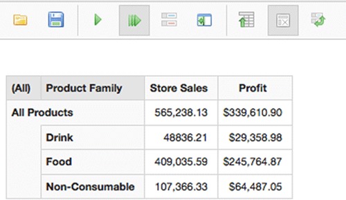
This is our data as it is now and represents what our cube tells us with no scenarios in play. This initial Saiku report represents our baseline.
Next, we’ll enable our ability to make changes to the data and create our Scenario for evaluation. In our example, we want to increase our sales by 5,000 from $48,836.21 to $53,836.21. To do so, we first start by clicking the Query Scenario button on the toolbar, typing in the new value (58836.21), and pressing Return (see figure 11.16). At this point, Saiku has enabled the scenario, given the changed value to Mondrian, and Mondrian is ready to rerun the MDX query with the modified values. We’d expect to see the value we just changed retain its +5000 value, but we’d also expect to see our totals and other calculated members changed in other spots as well.
Figure 11.16. Saiku scenario change

Figure 11.17 shows that, as expected, the figures for the [Store Sales] totals and [Profit] have adjusted by the 5,000 change we made to [Drink] for [1997]. What’s also worth noting is that [Profit], which is a calculated member, has also adjusted. This means that Mondrian is not just updating the base figures, but when connected with this scenario, it’s ensuring the results of all calculations also reflect that scenario change.
Figure 11.17. Saiku scenario result

Though calculated members do reflect the changes made to it in a scenario, they themselves can’t be changed. In our example, we can’t change [Profit] because it’s a calculated member; we can only change a value that’s a core measure aggregated from the database.
In our example, we saw the results of reflecting the change of a lower level in a hierarchy ([Drink]) on the total ([All Products]). But it’s also common to explore scenarios where you’d like to change the overall totals by 5,000 and see what requirements that places on the individual product family sales. Mondrian also supports this; it’s common for budget and planning workflows to look at year totals, then have those spread down to the month-by-month expenditures, and so on. Mondrian scenario support even allows various options on how the change is allocated to children (weighted allocation, weighted increment, equal allocation, and equal increment).
Scenario support in Saiku and Pentaho Analyzer
Currently Saiku is the only visual client to Mondrian that supports Scenarios. Scenarios aren’t available via XMLA either; only OLAP4J has support for using scenarios.
Pentaho Analyzer currently has no support for Scenarios whatsoever; scenario support is not currently in a planned Pentaho Analyzer release.
Lastly, there exists a requirement to create a hanger dimension to allow the scenarios to be used in MDX. Refer to section 5.4.2 for more information on how to define a hanger dimension. Readers are advised to look at the Saiku sample Mondrian schema files for the Sales Scenario cube for a working example of creating this hanger dimension for use with scenarios.
Now that we’ve looked at how to do what-if analysis with Mondrian, we’ll look at how to do some real high-powered data mining (DM) and machine learning (ML) using tools that specialize in this analysis.
11.3. Statistics and machine learning
Now that we’ve looked at some of the statistics you can do inside Mondrian (using MDX) and the ability to explore what-if scenarios, let’s explore what companies like Adventure Works do when they need more advanced statistics or machine learning. For instance, though MDX helps understand growth, ratios, and simple linear regressions, it’s nearly impossible to do a forecasting algorithm that includes commonly needed bounds and confidence intervals. For instance, what are the upper and lower bounds of my predicted sales figure with 95% confidence? These DM and ML packages help answer questions that Mondrian doesn’t endeavor to; they’re complementary.
Let’s explore, at a high level, some common use cases that would best be addressed with DM or ML packages:
- Predicting future values with ranges and confidence figures using regression and other techniques
- Clustering of similar customers together to segment customers by similar behavior and attributes
- Market-basket analysis to determine which items are often purchased together, even if they seem unrelated
- Fraud detection and analysis to determine outliers or unusual behavior
- Classic statistical descriptions of confidence in values such as the + or - 3% qualifiers typically seen in polls based on sample sizing
Mondrian doesn’t have any integrations directly with any data mining (DM) or machine learning (ML) packages. The approaches we cover here include how these systems are used in combination to create the end result functional requirements. This approach is not only the only practical method of integrations, but most users tend to find it perfectly reasonable and even preferable.
The most common method of combining Mondrian and DM tools is by simply using them on the same data. This is most often, and easily, achieved by using the different tools on the same source data. Mondrian uses a star schema (chapter 3) as the source for its multidimensional data, which also makes a perfectly good source for DM tools. This common approach makes sense: most of a company’s investment in building an analytic solution involves data integration, restructuring, and loading (ETL and modeling) into the database. Using the ETL and modeling work along with data enriched with additional lookup attributes is a great source for DM tools.
Data mining purists on star schemas
Data mining purists may disagree that the star schema, cleaned and loaded from original source, represents the best data to perform machine learning and data mining on. Why? With one level of cleanup and enrichment (fitting into categories and hierarchies), correcting data quality issues introduces some level of bias/effect on the data. Though this is true, in practice, DM practitioners often do some level of data preparation themselves for their modeling and do some similar things. Though not perfect, DM on star schemas (and their various aggregations/samples) is common, especially when the DM tool is to be used alongside Mondrian.
We’ll cover, at a very high level, two data mining tools commonly used in conjunction with Mondrian solutions and when to use them. The tools, R and Weka, are also open source themselves, which is part of the reason they’re so often used with Mondrian.
11.3.1. R
R is a language and environment for statistical computing and graphics (http://www.r-project.org/about.html). It’s a widely and commonly used package for data preparation, modeling, and statistical analysis. That’s worth noting: R is a language and set of tools that focus on statistics. It excels at classifying items, clustering like items together, and developing forecasts with confidence intervals. It’s the “go to” tool for many data scientists to use classic statistical methods on their dataset.
Like previously mentioned, the most common method for using R with Mondrian is to use them side by side. You can download the R software, including the UI, connect it to your database, retrieve sets of data, and then continue the analysis in R. It’s not necessary, or even that beneficial, to think of R connecting directly to Mondrian, since R tends to want to see the base level. In some cases, R (or the users of) would like to see some level of aggregation on raw events; in that case, it makes sense to point R at the aggregate tables inside the database already prepared for Mondrian performance (see section 7.3 for more on Mondrian aggregate tables).
An extensive community supports the R tool, including some commercial companies that offer support packages. R is primarily for statistics, but it also does have some capabilities for machine learning; there’s some overlap between R and Weka. You should choose whichever package fits your DM or ML needs in general. If you’re not sure, and you’re looking for more statistical based algorithms and don’t require any operational integration with Pentaho Data Integration, choose R. If you’re looking for a greater focus on machine learning algorithms or need operational integration with PDI, you should consider Weka, which we’ll discuss next.
11.3.2. Weka
Weka is a machine learning framework and tool (see figure 11.18). Similar to R, it provides UI tools for acquiring, managing, and filtering data for modeling. Models are built and evaluated using a dataset from a variety of data sources. Weka can use the star schema that any DM tool can access (like R), but it also has the advantage of being integrated into PDI as a series of useful plugins for doing common tasks. More on that later in this section.
Figure 11.18. Weka clustering output

Weka excels and is best known for its capabilities on machine learning algorithms. It’s well known for its large catalog of classification techniques, given its providence as a university project. Many researchers use Weka as their tool of choice for testing new algorithms, so there’s no shortage of available supervised and unsupervised learning algorithms. In fact, this large volume of available techniques and algorithms is sometimes daunting to those new to data mining.
Given the specialized knowledge of data mining, it’s difficult to get started. By far, the easiest way to get started with Weka is to use the prepackaged plugins available in Pentaho Data Integration to do common DM tasks. By using the PDI plugins to do some time-series forecasting and market-basket analysis, you’ll learn the basics of DM without extensive training. For the common use cases that are deployed alongside Mondrian, that’s a great way to start. With PDI’s ability to query Mondrian (http://wiki.pentaho.com/display/EAI/Mondrian+Input) and stream results to further steps, this is the closest direct integration between Mondrian and a DM tool.
Hopefully you have a good sense of the tools available to use in conjunction with Mondrian for more advanced data mining and machine learning use cases. It should be clear how R and Weka fit in an overall solution with Mondrian; we’ll now delve into a very Big (pun intended) topic and see where Mondrian fits in the Big Data space.
11.4. Big Data
Big Data, and the various technologies and skills involved, have garnered much attention in the past couple of years. These tools and technologies, the companies that produce them, and the practitioners that use them represent a huge segment of businesses that are looking to handle data that has
- Volume —Adventure Works needs to handle data volumes, where the total number of records they will manage two years from now will be more than 10x the data they manage now. The traditional databases they used to build their applications and analytic systems won’t always do so effectively on billions of records.
- Variety —Adventure Works will need to get data from existing corporate documents, NoSQL data stores, online resources, and multiple applications within the firewall. Gone are the days of applications storing things solely in relational SQL databases, but there exists an increasing amount of unstructured (or hierarchically structured) data.
- Velocity —Adventure Works needs to handle a constant and increasing stream of data, and time to analyze and present that data is shrinking. Things are happening faster on both the processing of records and analysis side.
Mondrian is a nice complement and is used in conjunction with Big Data tools constantly. Mondrian is, in its own way, a Big Data tool. It helps customers analyze large amounts of data (caching, aggregate tables), do analysis on varied types of data (your dimensions and metrics are your own), and allows near-real-time analysis with some advanced cache management APIs (see section 7.4 for more on caching and APIs). Mondrian’s focus on the OLAP space specifically, and leaving the heavy duty storage and aggregation to an RDBMS (see section 2.4.1 for more on ROLAP), provides significant benefit for nearly all companies; it’s easy to find a relational database in use somewhere in a company. This reliance on a SQL RDBMS does tie Mondrian closely with SQL data storage systems and limits the data stores that Mondrian can use directly to those that speak SQL.
Mondrian needs SQL
Mondrian requires a database that speaks SQL to work properly. Even if your back-end database has the same capabilities through an API (filtering, aggregation by fields, and so forth), it can’t be plugged in behind Mondrian. Users looking for connecting their NoSQL system with Mondrian should consider the work being undertaken at the Optiq project. Optiq is for creating a SQL layer on top of any data source (requiring a developer to write only the specific implementation) and is a practical method to connect Mondrian with a non-SQL source. Julian Hyde, coauthor of this book and lead developer of Mondrian, is also the project lead for Optiq (https://github.com/julianhyde/optiq).
11.4.1. Analytic databases
Mondrian fits with many Big Data systems that speak SQL. In particular, there’s an entire breed of databases that use SQL as their interface but have specialized storage and processing methods for analytics. These systems are typically column-oriented (store like data together) and often include the ability to scale out to multiple servers. Mondrian is known to work with the following analytic databases:
|
These databases are purpose-built for performing a workload very compatible with Mondrian. Mondrian generates many SQL statements to run in the RDBMS, from dimension lookups to aggregation plus group by SQL statements. These databases are purpose-built to execute the exact type of query that Mondrian generates. Though Mondrian will work with adequate performance on most traditional OLTP databases (Oracle, MySQL, PostGres, and so on), it’ll perform much faster, and certainly much faster with more data, on an analytic database.
11.4.2. Hadoop and Hive
Hadoop is a very popular system for doing data processing; as a framework, it addresses all the V’s (volume, variety, and velocity) as part of a large open source community. Hive is a SQL layer on top of Hadoop that allows users to run a SQL-like syntax on top of HDFS and Hadoop data. This provides significant benefit to Hadoop users performing an analytic workload on top of Hadoop. Mondrian has experimental support for Hive and will work functionally on top of Hive soon.
But unless a system like Cloudera’s Impala or an additional query latency improvement system is also utilized, Adventure Works would likely be disappointed with the performance of Mondrian on top of Hive. Mondrian often issues many SQL queries to a database to look up dimension members, children, and get aggregations. Hive experiences high latency with often simple queries as well (5–10s); Mondrian makes an assumption that some queries run fast (lookup members in a dimension) while the aggregations hitting facts are slow.
Hadoop/Hive support
Hive support is being developed; even if Mondrian is functional on top of Hive, the latency for dimension member and similar lookups is a challenge for making an overall high-performance OLAP system with Mondrian and Hive.
Though Hive is a popular way to access data in Hadoop, there are other ways of using Hadoop and Mondrian together. When Hadoop is used, without Hive, it looks similar to the general NoSQL approaches we cover next.
11.4.3. NoSQL systems and Hadoop
Mondrian, being a system which requires SQL and a whole new class of systems that don’t speak SQL (NoSQL = Not Only SQL), creates a natural question for Adventure Works: How do these things work together? Adventure Works has a mobile application that uses Cloudant (a hosted version of CouchDB) for storage; it’s a popular document-based storage service for mobile developers. Adventure Works needs to do some reporting on a huge amount of documents stored in Cloudant, and Mondrian matches the reporting needs of the users.
Two methods are available to Adventure Works to use Mondrian on data in this NoSQL system. One is extremely common, not terribly sophisticated, and gets the job done today using a SQL database in between. The second is a sophisticated and cutting-edge technique to put a SQL driver in front of any system or API. We’ll cover both approaches here.
NoSQL as a distributed cache
It’s worth mentioning that the two techniques covered in this section explore using NoSQL as the primary source for data in Mondrian. There’s another technique that integrates NoSQL technology into Mondrian, but not as the primary storage and aggregation engine. NoSQL systems have been used by the pluggable cache API to allow Mondrian to share its cache among individual servers in a multiserver environment. Though this might not help users do reporting on top of NoSQL, it can certainly leverage some of the fantastic key value scalability and performance for managing Mondrian’s cache (see section 7.4.2 for more on using an external segment cache).
ETL data into SQL database
This is the most common solution in practice today; for those who want to do ad hoc, high-performance analytics on top of data with NoSQL and Mondrian, the solution isn’t really one at all. Adventure Works can take the data in CouchDB, run a periodic ETL process to capture the relevant data for the analytic solution, and push that data into a SQL database. Once in the database, Mondrian performs its analysis on top of the data, without modification or need to connect with the NoSQL system, as shown in figure 11.19. Most users will only export some sort of first-level sort and aggregation to reduce the dataset to the daily (or hourly) aggregations at the lowest level of aggregation.
Figure 11.19. NoSQL plus database architecture

There are some advantages to this approach. First is that the technologies involved are all mature, with years of deployment knowledge and experience. Second is that it has the same virtue as the traditional DW in that it offloads the analytic processing (which is different) to another system. It reduces the load on the source systems and separates out different kinds of use cases and workload.
There are also some disadvantages. The data is now stored separately, and there’s an inherent staleness to data from the NoSQL system and the data presented to Adventure Works users. Another disadvantage is that some of these NoSQL systems are very scalable and handle the storage and aggregation as good as or better than their RDBMS peers. In other words, we could leverage some great, free, and open source technology to act as the primary aggregation engine for our Mondrian solution, but we’re simply putting it back into a less scalable SQL database.
SQL access to NoSQL systems
This is the less commonly used approach; similar in approach to accessing Hadoop data via Hive, this approach suggests that creating a way to “speak SQL” to NoSQL systems is interesting and is being used by many commercial tools. There’s even an up-and-coming open source project being developed by an author of this book (Julian Hyde) providing a general JDBC driver for any system.
Speaking SQL to a NoSQL system has some advantages. SQL is a widely known language; its dominance in BI tools is unmistakable, and Mondrian is no exception. If a NoSQL system can offer the basic semantics that Mondrian SQL requires (filtering, grouping, and aggregation), then it can act as the primary storage and aggregation engine in Adventure Works’ solution. Some of these NoSQL solutions do this (or are very close) and provide some remarkable scaling and performance compared to their RDBMS peers.
It’s not without some drawbacks as well; you lose some of the richness of the native API for the NoSQL system. SQL, in particular the SQL Mondrian generates, represents a “least common denominator” for accessing data in a data store. The NoSQL systems often offer additional capabilities (intermediate group results in hierarchies) that aren’t expressed in Mondrian SQL.
11.5. Summary
In this chapter we’ve looked at how we can do advanced ratios, percentages, and time-based calculations in Mondrian. This provides Adventure Works a basis for calculating many advanced analytics inside Mondrian with great speed and efficiency. We then looked at how Mondrian and Saiku can support basic “What If” analysis, making changes on the fly to see the effects of different scenarios.
We then continued to see what options Adventure Works has if they’re looking to do more advanced data mining and machine learning. We introduced R and Weka, the most commonly used tools with Mondrian. Lastly we helped place Mondrian in the proliferation of new technologies wrapped in the Big Data moniker. We introduced how Mondrian is currently being used as, and in conjunction with, Big Data systems.