
R has a reputation for being slow and memory-inefficient, a reputation that is at least somewhat earned. These faults are largely unnoticed on a modern PC for datasets of many thousands of records, but datasets with a million records or more can exceed the limits of what is currently possible with consumer-grade hardware. The problem worsens if the dataset contains many features or if complex learning algorithms are being used.
Note
CRAN has a high-performance computing task view that lists packages pushing the boundaries of what is possible in R. It can be viewed at http://cran.r-project.org/web/views/HighPerformanceComputing.html.
Packages that extend R past the capabilities of the base software are being developed rapidly. This work comes primarily on two fronts: some packages add the capability to manage extremely large datasets by making data operations faster or allowing the size of the data to exceed the amount of available system memory; others allow R to work faster, perhaps by spreading the work over additional computers or processors, utilizing specialized computer hardware, or providing machine learning algorithms optimized for big data problems.
Extremely large datasets can cause R to grind to a halt when the system runs out of memory to store data. Even if the entire dataset can fit into the available memory, additional memory overhead will be needed for data processing. Furthermore, very large datasets can take a long amount of time to analyze for no reason other than the sheer volume of records; even a quick operation can cause delays when performed many millions of times.
Years ago, many would perform data preparation outside R in another programming language, or use R but perform analyses on a smaller subset of data. However, this is no longer necessary, as several packages have been contributed to R to address these problems.
The dplyr package introduced in 2014 by Hadley Wickham and Romain Francois is perhaps the most straightforward way to begin working with large datasets in R. Though other packages may exceed its capabilities in terms of raw speed or the raw size of the data, dplyr is still quite capable. More importantly, it is virtually transparent after the initial learning curve has passed.
Note
For more information on dplyr, including some very helpful tutorials, refer to the project's GitHub page at https://github.com/hadley/dplyr.
Put simply, the package provides an object called tbl, which is an abstraction of tabular data. It acts much like a data frame, with several important exceptions:
- Key functionality has been written in C++, which according to the authors results in a 20x to 1000x performance increase for many operations.
- R data frames are limited by available memory. The
dplyrversion of a data frame can be linked transparently to disk-based databases that can exceed what can be stored in memory. - The
dplyrpackage makes reasonable assumptions about data frames that optimize your effort as well as memory use. It doesn't automatically change data types. And, if possible, it avoids making copies of data by pointing to the original value instead. - New operators are introduced that allow common data transformations to be performed with much less code while remaining highly readable.
Making the transition from data frames to dplyr is easy. To convert an existing data frame into a tbl object, use the as.tbl() function:
> library(dplyr)
> credit <- read.csv("credit.csv")
> credit_tbl <- as.tbl(credit)
Typing the name of the table provides information about the object. Even here, we see a distinction between dplyr and typical R behavior; where as a traditional data frame would have displayed many rows of data, dplyr objects are more considerate of real-world needs. For example, typing the name of the object provides output summarized in a form that fits a single screen:
> credit_tbl

Connecting dplyr to an external database is straightforward as well. The dplyr package provides functions to connect to MySQL, PostgreSQL, and SQLite databases. These create a connection object that allows tbl objects to be pulled from the database.
Let's use the src_sqlite() function to create a SQLite database to store credit data. SQLite is a simple database that doesn't require a server. It simply connects to a database file, which we'll call credit.sqlite3. Since the file doesn't exist yet, we need to set the create = TRUE parameter to create the file. Note that for this step to work, you may require to install the RSQLite package if you have not already done so:
> credit_db_conn <- src_sqlite("credit.sqlite3", create = TRUE)
After creating the connection, we need to load the data into the database using the copy_to() function. This uses the credit_tbl object to create a database table within the database specified by credit_db_conn. The temporary = FALSE parameter forces the table to be created immediately. Since dplyr tries to avoid copying data unless it must, it will only create the table if it is explicitly asked to:
> copy_to(credit_db_conn, credit_tbl, temporary = FALSE)
Executing the copy_to() function will store the data in the credit.sqlite3 file, which can be transported to other systems as needed. To access this file later, simply reopen the database connection and create a tbl object, as follows:
> credit_db_conn <- src_sqlite("credit.sqlite3")
> credit_tbl <- tbl(credit_db_conn, "credit_tbl")
In spite of the fact that dplyr is routed through a database, the credit_tbl object here will act exactly like any other tbl object and will gain all the other benefits of the dplyr package.
The data.table package by Matt Dowle, Tom Short, Steve Lianoglou, and Arun Srinivasan provides an enhanced version of a data frame called a data table. The data.table objects are typically much faster than data frames for subsetting, joining, and grouping operations. For the largest datasets—those with many millions of rows—these objects may be substantially faster than even dplyr objects. Yet, because it is essentially an improved data frame, the resulting objects can still be used by any R function that accepts a data frame.
Note
The data.table project can be found on GitHub at https://github.com/Rdatatable/data.table/wiki.
After installing the data.table package, the fread() function will read tabular files like CSVs into data table objects. For instance, to load the credit data used previously, type:
> library(data.table)
> credit <- fread("credit.csv")
The credit data table can then be queried using syntax similar to R's [row, col] form, but optimized for speed and some additional useful conveniences. In particular, the data table structure allows the row portion to select rows using an abbreviated subsetting command, and the col portion to use a function that does something with the selected rows. For example, the following command computes the mean requested loan amount for people with a good credit history:
> credit[credit_history == "good", mean(amount)]
[1] 3040.958
By building larger queries with this simple syntax, very complex operations can be performed on data tables. Since the data structure is optimized for speed, it can be used with large datasets.
One limitation of the data.table structures is that like data frames they are limited by the available system memory. The next two sections discuss packages that overcome this shortcoming at the expense of breaking compatibility with many R functions.
Tip
The dplyr and data.table packages each have unique strengths. For an in-depth comparison, check out the following Stack Overflow discussion at http://stackoverflow.com/questions/21435339/data-table-vs-dplyr-can-one-do-something-well-the-other-cant-or-does-poorly. It is also possible to have the best of both worlds, as data.table structures can be loaded into dplyr using the tbl_dt() function.
The ff package by Daniel Adler, Christian Gläser, Oleg Nenadic, Jens Oehlschlägel, and Walter Zucchini provides an alternative to a data frame (ffdf) that allows datasets of over two billion rows to be created, even if this far exceeds the available system memory.
The ffdf structure has a physical component that stores the data on a disk in a highly efficient form, and a virtual component that acts like a typical R data frame, but transparently points to the data stored in the physical component. You can imagine the ffdf object as a map that points to a location of the data on a disk.
Note
The ff project is on the Web at http://ff.r-forge.r-project.org/.
A downside of ffdf data structures is that they cannot be used natively by most R functions. Instead, the data must be processed in small chunks, and the results must be combined later on. The upside of chunking the data is that the task can be divided across several processors simultaneously using the parallel computing methods presented later in this chapter.
After installing the ff package, to read in a large CSV file, use the read.csv.ffdf() function, as follows:
> library(ff)
> credit <- read.csv.ffdf(file = "credit.csv", header = TRUE)
Unfortunately, we cannot work directly with the ffdf object, as attempting to treat it like a traditional data frame results in an error message:
> mean(credit$amount)
[1] NA
Warning message:
In mean.default(credit$amount) :
  argument is not numeric or logical: returning NA
The ffbase package by Edwin de Jonge, Jan Wijffels, and Jan van der Laan addresses this issue somewhat by adding capabilities for basic analyses using ff objects. This makes it possible to use ff objects directly for data exploration. For instance, after installing the ffbase package, the mean function works as expected:
> library(ffbase)
> mean(credit$amount)
[1] 3271.258
The package also provides other basic functionality such as mathematical operators, query functions, summary statistics, and wrappers to work with optimized machine learning algorithms like biglm (described later in this chapter). Though these do not completely eliminate the challenges of working with extremely large datasets, they make the process a bit more seamless.
Note
For more information on advanced functionality, visit the ffbase project site at http://github.com/edwindj/ffbase.
The bigmemory package by Michael J. Kane, John W. Emerson, and Peter Haverty allows the use of extremely large matrices that exceed the amount of available system memory. The matrices can be stored on a disk or in shared memory, allowing them to be used by other processes on the same computer or across a network. This facilitates parallel computing methods, such as the ones covered later in this chapter.
Note
Additional documentation on the bigmemory package can be found at http://www.bigmemory.org/.
Because bigmemory matrices are intentionally unlike data frames, they cannot be used directly with most of the machine learning methods covered in this book. They also can only be used with numeric data. That said, since they are similar to a typical R matrix, it is easy to create smaller samples or chunks that can be converted into standard R data structures.
The authors also provide the bigalgebra, biganalytics, and bigtabulate packages, which allow simple analyses to be performed on the matrices. Of particular note is the bigkmeans() function in the biganalytics package, which performs k-means clustering as described in Chapter 9, Finding Groups of Data – Clustering with k-means. Due to the highly specialized nature of these packages, use cases are outside the scope of this chapter.
In the early days of computing, processors executed instructions in serial which meant that they were limited to performing a single task at a time. The next instruction could not be started until the previous instruction was complete. Although it was widely known that many tasks could be completed more efficiently by completing the steps simultaneously, the technology simply did not exist yet.

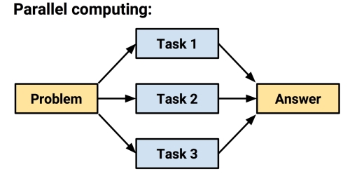
This was addressed by the development of parallel computing methods, which use a set of two or more processors or computers to solve a larger problem. Many modern computers are designed for parallel computing. Even in the cases in which they have a single processor, they often have two or more cores that are capable of working in parallel. This allows tasks to be accomplished independently of one another.
Networks of multiple computers called clusters can also be used for parallel computing. A large cluster may include a variety of hardware and be separated over large distances. In this case, the cluster is known as a grid. Taken to an extreme, a cluster or grid of hundreds or thousands of computers running commodity hardware could be a very powerful system.
The catch, however, is that not every problem can be parallelized. Certain problems are more conducive to parallel execution than others. One might expect that adding 100 processors would result in accomplishing 100 times the work in the same amount of time (that is, the overall execution time would be 1/100), but this is typically not the case. The reason is that it takes effort to manage the workers. Work must be divided into equal, nonoverlapping tasks, and each of the workers' results must be combined into one final answer.
So-called embarrassingly parallel problems are ideal. It is easy to reduce these tasks into nonoverlapping blocks of work and recombine the results. An example of an embarrassingly parallel machine learning task would be 10-fold cross-validation; once the 10 samples are divided, each of the 10 blocks of work is independent, meaning that they do not affect the others. As you will soon see, this task can be sped up quite dramatically using parallel computing.
Efforts to speed up R will be wasted if it is not possible to systematically measure how much time is saved. Although a stopwatch is one option, an easier solution would be to wrap the code in a system.time() function.
For example, on my laptop, the system.time() function notes that it takes about 0.093 seconds to generate a million random numbers:
> system.time(rnorm(1000000))
   user  system elapsed
  0.092   0.000   0.093
The same function can be used to evaluate the improvement in performance obtained by using the methods that were just described or any R function.
Note
For what it's worth, when the first edition was published, generating a million random numbers took 0.13 seconds. Although I'm now using a slightly more powerful computer, this reduction of about 30 percent of the processing time just two years later illustrates how quickly computer hardware and software are improving.
The parallel package, now included with R version 2.14.0 and higher, has lowered the entry barrier to deploy parallel algorithms by providing a standard framework to set up worker processes that can complete tasks simultaneously. It does this by including components of the multicore and snow packages, each taking a different approach towards multitasking.
If your computer is reasonably recent, you are likely to be able to use parallel processing. To determine the number of cores your machine has, use the detectCores() function as follows. Note that your output will differ depending on your hardware specifications:
> library(parallel)
> detectCores()
[1] 8
The multicore package was developed by Simon Urbanek and allows parallel processing on a single machine that has multiple processors or processor cores. It utilizes the multitasking capabilities of a computer's operating system to fork additional R sessions that share the same memory. It is perhaps the simplest way to get started with parallel processing in R. Unfortunately, because Windows does not support forking, this solution will not work everywhere.
An easy way to get started with the multicore functionality is to use the mclapply() function, which is a parallel version of lapply(). For instance, the following blocks of code illustrate how the task of generating a million random numbers can be divided across 1, 2, 4, and 8 cores. The unlist() function is used to combine the parallel results (a list) into a single vector after each core has completed its chunk of work:
> system.time(l1 <- rnorm(1000000))
   user  system elapsed
  0.094   0.003   0.097

> system.time(l2 <- unlist(mclapply(1:2, function(x) {
  rnorm(500000)}, mc.cores = 2)))
   user  system elapsed
  0.106   0.045   0.076

> system.time(l4 <- unlist(mclapply(1:4, function(x) {
  rnorm(250000) }, mc.cores = 4)))
   user  system elapsed
  0.135   0.055   0.063

> system.time(l8 <- unlist(mclapply(1:8, function(x) {
  rnorm(125000) }, mc.cores = 8)))
   user  system elapsed
  0.123   0.058   0.055
Notice how as the number of cores increases, the elapsed time decreases, and the benefit tapers off. Though this is a simple example, it can be adapted easily to many other tasks.
The snow package (simple networking of workstations) by Luke Tierney, A. J. Rossini, Na Li, and H. Sevcikova allows parallel computing on multicore or multiprocessor machines as well as on a network of multiple machines. It is slightly more difficult to use, but offers much more power and flexibility. After installing snow, to set up a cluster on a single machine, use the makeCluster() function with the number of cores to be used:
> library(snow)
> cl1 <- makeCluster(4)
Because snow communicates via network traffic, depending on your operating system, you may receive a message to approve access through your firewall.
To confirm whether the cluster is operational, we can ask each node to report back its hostname. The clusterCall() function executes a function on each machine in the cluster. In this case, we'll define a function that simply calls the Sys.info() function and returns the nodename parameter:
> clusterCall(cl1, function() { Sys.info()["nodename"] } )
[[1]]
                  nodename
"Bretts-Macbook-Pro.local"

[[2]]
                  nodename
"Bretts-Macbook-Pro.local"

[[3]]
                  nodename
"Bretts-Macbook-Pro.local"

[[4]]
                  nodename
"Bretts-Macbook-Pro.local"
Unsurprisingly, since all four nodes are running on a single machine, they report back the same hostname. To have the four nodes run a different command, supply them with a unique parameter via the clusterApply() function. Here, we'll supply each node with a different letter. Each node will then perform a simple function on its letter in parallel:
> clusterApply(cl1, c('A', 'B', 'C', 'D'),
               function(x) { paste("Cluster", x, "ready!") })
[[1]]
[1] "Cluster A ready!"

[[2]]
[1] "Cluster B ready!"

[[3]]
[1] "Cluster C ready!"

[[4]]
[1] "Cluster D ready!"
Once we're done with the cluster, it's important to terminate the processes it spawned. This will free up the resources each node is using:
> stopCluster(cl1)
Using these simple commands, it is possible to speed up many machine learning tasks. For larger big data problems, much more complex snow configurations are possible. For instance, you may attempt to configure a Beowulf cluster—a network of many consumer-grade machines. In academic and industry research settings with dedicated computing clusters, snow can use the Rmpi package to access these high-performance message-passing interface (MPI) servers. Working with such clusters requires the knowledge of network configurations and computing hardware, which is outside the scope of this book.
Note
For a much more detailed introduction to snow, including some information on how to configure parallel computing on several computers over a network, see http://homepage.stat.uiowa.edu/~luke/classes/295-hpc/notes/snow.pdf.
The foreach package by Steve Weston of Revolution Analytics provides perhaps the easiest way to get started with parallel computing, particularly if you are running R on Windows, as some of the other packages are platform-specific.
The core of the package is a new foreach looping construct. If you have worked with other programming languages, you may be familiar with it. Essentially, it allows looping over a number of items in a set without explicitly counting the number of items; in other words, for each item in the set, do something.
Note
In addition to the foreach package, Revolution Analytics (recently acquired by Microsoft) has developed high-performance, enterprise-ready R builds. Free versions are available for trial and academic use. For more information, see their website at http://www.revolutionanalytics.com/.
If you're thinking that R already provides a set of apply functions to loop over the sets of items (for example, apply(), lapply(), sapply(), and so on), you are correct. However, the foreach loop has an additional benefit: iterations of the loop can be completed in parallel using a very simple syntax. Let's see how this works.
Recall the command we've been using to generate a million random numbers:
> system.time(l1 <- rnorm(1000000))
   user  system elapsed
  0.096   0.000   0.096
After the foreach package has been installed, it can be expressed by a loop that generates four sets of 250,000 random numbers in parallel. The .combine parameter is an optional setting that tells foreach which function it should use to combine the final set of results from each loop iteration. In this case, since each iteration generates a set of random numbers, we simply use the c() concatenate function to create a single, combined vector:
> library(foreach)
> system.time(l4 <- foreach(i = 1:4, .combine = 'c')
                %do% rnorm(250000))
   user  system elapsed
  0.106   0.003   0.109
If you noticed that this function didn't result in a speed improvement, good catch! The reason is that by default, the foreach package runs each loop iteration in serial. The doParallel sister package provides a parallel backend for foreach that utilizes the parallel package included with R, which was described earlier in this chapter. After installing the doParallel package, simply register the number of cores and swap the %do% command with %dopar%, as follows:
> library(doParallel)
> registerDoParallel(cores = 4)
> system.time(l4p <- foreach(i = 1:4, .combine = 'c')
                       %dopar% rnorm(250000))
   user  system elapsed
  0.062   0.030   0.054
As shown in the output, this code results in the expected performance improvement, nearly cutting the execution time in half.
To close the doParallel cluster, simply type:
> stopImplicitCluster()
Though the cluster will be closed automatically at the conclusion of the R session, it is better form to do so explicitly.
The MapReduce programming model was developed at Google as a way to process their data on a large cluster of networked computers. MapReduce defined parallel programming as a two-step process:
A popular open source alternative to the proprietary MapReduce framework is Apache Hadoop. The Hadoop software comprises of the MapReduce concept, plus a distributed filesystem capable of storing large amounts of data across a cluster of computers.
Note
Packt Publishing has published a large number of books on Hadoop. To search current offerings, visit https://www.packtpub.com/all/?search=hadoop.
Several R projects that provide an R interface to Hadoop are in development. The RHadoop project by Revolution Analytics provides an R interface to Hadoop. The project provides a package, rmr, intended to be an easy way for R developers to write MapReduce programs. Another companion package, plyrmr, provides functionality similar to the dplyr package to process large datasets. Additional RHadoop packages provide R functions to access Hadoop's distributed data stores.
Note
For more information on the RHadoop project, see https://github.com/RevolutionAnalytics/RHadoop/wiki.
Another similar project is RHIPE by Saptarshi Guha, which attempts to bring Hadoop's divide and recombine philosophy into R by managing the communication between R and Hadoop.
Note
The RHIPE package is not yet available at CRAN, but it can be built from the source available on the Web at http://www.datadr.org.
An alternative to parallel processing uses a computer's Graphics Processing Unit (GPU) to increase the speed of mathematical calculations. A GPU is a specialized processor that is optimized to rapidly display images on a computer screen. Because a computer often needs to display complex 3D graphics (particularly for video games), many GPUs use hardware designed for parallel processing and extremely efficient matrix and vector calculations. A side benefit is that they can be used to efficiently solve certain types of mathematical problems. Where a computer processor may have 16 cores, a GPU may have thousands.

The downside of GPU computing is that it requires specific hardware that is not included in many computers. In most cases, a GPU from the manufacturer Nvidia is required, as they provide a proprietary framework called Complete Unified Device Architecture (CUDA) that makes the GPU programmable using common languages such as C++.
Note
For more information on Nvidia's role in GPU computing, go to http://www.nvidia.com/object/what-is-gpu-computing.html.
The gputools package by Josh Buckner, Mark Seligman, and Justin Wilson implements several R functions, such as matrix operations, clustering, and regression modeling using the Nvidia CUDA toolkit. The package requires a CUDA 1.3 or higher GPU and the installation of the Nvidia CUDA toolkit.
Some of the machine learning algorithms covered in this book are able to work on extremely large datasets with relatively minor modifications. For instance, it would be fairly straightforward to implement Naive Bayes or the Apriori algorithm using one of the data structures for big datasets described in the previous sections. Some types of learners, such as ensembles, lend themselves well to parallelization, because the work of each model can be distributed across processors or computers in a cluster. On the other hand, some require larger changes to the data or algorithm, or need to be rethought altogether, before they can be used with massive datasets.
The following sections examine packages that provide optimized versions of the learning algorithms we've worked with so far.
The biglm package by Thomas Lumley provides functions to train regression models on datasets that may be too large to fit into memory. It works by using an iterative process in which the model is updated little by little using small chunks of data. In spite of it being a different approach, the results will be nearly identical to what would be obtained by running the conventional lm() function on the entire dataset.
For convenience while working with the largest datasets, the biglm() function allows the use of a SQL database in place of a data frame. The model can also be trained with chunks obtained from data objects created by the ff package described previously.
The bigrf package by Aloysius Lim implements the training of random forests for classification and regression on datasets that are too large to fit into memory. It uses the bigmemory objects as described earlier in this chapter. For speedier forest growth, the package can be used with the foreach and doParallel packages described previously to grow trees in parallel.
Note
For more information, including examples and Windows installation instructions, see the package's wiki, which is hosted on GitHub at https://github.com/aloysius-lim/bigrf.
The caret package by Max Kuhn (covered extensively in Chapter 10, Evaluating Model Performance and Chapter 11, Improving Model Performance) will transparently utilize a parallel backend if one has been registered with R using the foreach package described previously.
Let's take a look at a simple example in which we attempt to train a random forest model on the credit dataset. Without parallelization, the model takes about 109 seconds to be trained:
> library(caret)
> credit <- read.csv("credit.csv")
> system.time(train(default ~ ., data = credit, method = "rf"))
   user  system elapsed
107.862   0.990 108.873
On the other hand, if we use the doParallel package to register the four cores to be used in parallel, the model takes under 32 seconds to build—less than a third of the time—and we didn't need to change even a single line of the caret code:
> library(doParallel)
> registerDoParallel(cores = 4)
> system.time(train(default ~ ., data = credit, method = "rf"))
   user  system elapsed
114.578   2.037  31.362
Many of the tasks involved in training and evaluating models, such as creating random samples and repeatedly testing predictions for 10-fold cross-validation are embarrassingly parallel and ripe for performance improvements. With this in mind, it is wise to always register multiple cores before beginning a caret project.
Note
Configuration instructions and a case study of the performance improvements needed to enable parallel processing in caret are available on the project's website at http://topepo.github.io/caret/parallel.html.