
Interacting with friends on a social networking service (SNS), such as Facebook, Tumblr, and Instagram has become a rite of passage for teenagers around the world. Having a relatively large amount of disposable income, these adolescents are a coveted demographic for businesses hoping to sell snacks, beverages, electronics, and hygiene products.
The many millions of teenage consumers using such sites have attracted the attention of marketers struggling to find an edge in an increasingly competitive market. One way to gain this edge is to identify segments of teenagers who share similar tastes, so that clients can avoid targeting advertisements to teens with no interest in the product being sold. For instance, sporting apparel is likely to be a difficult sell to teens with no interest in sports.
Given the text of teenagers' SNS pages, we can identify groups that share common interests such as sports, religion, or music. Clustering can automate the process of discovering the natural segments in this population. However, it will be up to us to decide whether or not the clusters are interesting and how we can use them for advertising. Let's try this process from start to finish.
For this analysis, we will use a dataset representing a random sample of 30,000 U.S. high school students who had profiles on a well-known SNS in 2006. To protect the users' anonymity, the SNS will remain unnamed. However, at the time the data was collected, the SNS was a popular web destination for US teenagers. Therefore, it is reasonable to assume that the profiles represent a fairly wide cross section of American adolescents in 2006.
Tip
This dataset was compiled by Brett Lantz while conducting sociological research on the teenage identities at the University of Notre Dame. If you use the data for research purposes, please cite this book chapter. The full dataset is available at the Packt Publishing website with the filename snsdata.csv. To follow along interactively, this chapter assumes that you have saved this file to your R working directory.
The data was sampled evenly across four high school graduation years (2006 through 2009) representing the senior, junior, sophomore, and freshman classes at the time of data collection. Using an automated web crawler, the full text of the SNS profiles were downloaded, and each teen's gender, age, and number of SNS friends was recorded.
A text mining tool was used to divide the remaining SNS page content into words. From the top 500 words appearing across all the pages, 36 words were chosen to represent five categories of interests: namely extracurricular activities, fashion, religion, romance, and antisocial behavior. The 36 words include terms such as football, sexy, kissed, bible, shopping, death, and drugs. The final dataset indicates, for each person, how many times each word appeared in the person's SNS profile.
We can use the default settings of read.csv() to load the data into a data frame:
> teens <- read.csv("snsdata.csv")
Let's also take a quick look at the specifics of the data. The first several lines of the str() output are as follows:
> str(teens)
'data.frame':  30000 obs. of  40 variables:
 $ gradyear    : int  2006 2006 2006 2006 2006 2006 2006 2006 ...
 $ gender      : Factor w/ 2 levels "F","M": 2 1 2 1 NA 1 1 2 ...
 $ age         : num  19 18.8 18.3 18.9 19 ...
 $ friends     : int  7 0 69 0 10 142 72 17 52 39 ...
 $ basketball  : int  0 0 0 0 0 0 0 0 0 0 ...
As we had expected, the data include 30,000 teenagers with four variables indicating personal characteristics and 36 words indicating interests.
Do you notice anything strange around the gender row? If you were looking carefully, you may have noticed the NA value, which is out of place compared to the 1 and 2 values. The NA is R's way of telling us that the record has a missing value—we do not know the person's gender. Until now, we haven't dealt with missing data, but it can be a significant problem for many types of analyses.
Let's see how substantial this problem is. One option is to use the table() command, as follows:
> table(teens$gender)
    F     M
22054  5222
Although this command tells us how many F and M values are present, the table() function excluded the NA values rather than treating it as a separate category. To include the NA values (if there are any), we simply need to add an additional parameter:
> table(teens$gender, useNA = "ifany")
    F     M  <NA>
22054  5222  2724
Here, we see that 2,724 records (9 percent) have missing gender data. Interestingly, there are over four times as many females as males in the SNS data, suggesting that males are not as inclined to use SNS websites as females.
If you examine the other variables in the data frame, you will find that besides gender, only age has missing values. For numeric data, the summary() command tells us the number of missing NA values:
> summary(teens$age)
   Min. 1st Qu.  Median    Mean 3rd Qu.    Max.    NA's
  3.086  16.310  17.290  17.990  18.260 106.900    5086
A total of 5,086 records (17 percent) have missing ages. Also concerning is the fact that the minimum and maximum values seem to be unreasonable; it is unlikely that a 3 year old or a 106 year old is attending high school. To ensure that these extreme values don't cause problems for the analysis, we'll need to clean them up before moving on.
A more reasonable range of ages for the high school students includes those who are at least 13 years old and not yet 20 years old. Any age value falling outside this range should be treated the same as missing data—we cannot trust the age provided. To recode the age variable, we can use the ifelse() function, assigning teen$age the value of teen$age if the age is at least 13 and less than 20 years; otherwise, it will receive the value NA:
> teens$age <- ifelse(teens$age >= 13 & teens$age < 20,
                        teens$age, NA)
By rechecking the summary() output, we see that the age range now follows a distribution that looks much more like an actual high school:
> summary(teens$age)
   Min. 1st Qu.  Median    Mean 3rd Qu.    Max.    NA's
  13.03   16.30   17.26   17.25   18.22   20.00    5523
Unfortunately, now we've created an even larger missing data problem. We'll need to find a way to deal with these values before continuing with our analysis.
An easy solution for handling the missing values is to exclude any record with a missing value. However, if you think through the implications of this practice, you might think twice before doing so—just because it is easy does not mean it is a good idea! The problem with this approach is that even if the missingness is not extensive, you can easily exclude large portions of the data.
For example, suppose that in our data, the people with the NA values for gender are completely different from those with missing age data. This would imply that by excluding those missing either gender or age, you would exclude 9% + 17% = 26% of the data, or over 7,500 records. And this is for missing data on only two variables! The larger the number of missing values present in a dataset, the more likely it is that any given record will be excluded. Fairly soon, you will be left with a tiny subset of data, or worse, the remaining records will be systematically different or non-representative of the full population.
An alternative solution for categorical variables like gender is to treat a missing value as a separate category. For instance, rather than limiting to female and male, we can add an additional category for the unknown gender. This allows us to utilize dummy coding, which was covered in Chapter 3, Lazy Learning – Classification Using Nearest Neighbors.
If you recall, dummy coding involves creating a separate binary (1 or 0) valued dummy variable for each level of a nominal feature except one, which is held out to serve as the reference group. The reason one category can be excluded is because its status can be inferred from the other categories. For instance, if someone is not female and not unknown gender, they must be male. Therefore, in this case, we need to only create dummy variables for female and unknown gender:
> teens$female <- ifelse(teens$gender == "F" &
                           !is.na(teens$gender), 1, 0)
> teens$no_gender <- ifelse(is.na(teens$gender), 1, 0)
As you might expect, the is.na() function tests whether gender is equal to NA. Therefore, the first statement assigns teens$female the value 1 if gender is equal to F and the gender is not equal to NA; otherwise, it assigns the value 0. In the second statement, if is.na() returns TRUE, meaning the gender is missing, the teens$no_gender variable is assigned 1; otherwise, it is assigned the value 0. To confirm that we did the work correctly, let's compare our constructed dummy variables to the original gender variable:
> table(teens$gender, useNA = "ifany")
    F     M  <NA>
22054  5222  2724
> table(teens$female, useNA = "ifany")
    0     1
 7946 22054
> table(teens$no_gender, useNA = "ifany")
    0     1
27276  2724
The number of 1 values for teens$female and teens$no_gender matches the number of F and NA values, respectively, so we should be able to trust our work.
Next, let's eliminate the 5,523 missing age values. As age is numeric, it doesn't make sense to create an additional category for the unknown values—where would you rank "unknown" relative to the other ages? Instead, we'll use a different strategy known as imputation, which involves filling in the missing data with a guess as to the true value.
Can you think of a way we might be able to use the SNS data to make an informed guess about a teenager's age? If you are thinking of using the graduation year, you've got the right idea. Most people in a graduation cohort were born within a single calendar year. If we can identify the typical age for each cohort, we would have a fairly reasonable estimate of the age of a student in that graduation year.
One way to find a typical value is by calculating the average or mean value. If we try to apply the mean() function, as we did for previous analyses, there's a problem:
> mean(teens$age)
[1] NA
The issue is that the mean is undefined for a vector containing missing data. As our age data contains missing values, mean(teens$age) returns a missing value. We can correct this by adding an additional parameter to remove the missing values before calculating the mean:
> mean(teens$age, na.rm = TRUE)
[1] 17.25243
This reveals that the average student in our data is about 17 years old. This only gets us part of the way there; we actually need the average age for each graduation year. You might be tempted to calculate the mean four times, but one of the benefits of R is that there's usually a way to avoid repeating oneself. In this case, the aggregate() function is the tool for the job. It computes statistics for subgroups of data. Here, it calculates the mean age by graduation year after removing the NA values:
> aggregate(data = teens, age ~ gradyear, mean, na.rm = TRUE)
  gradyear      age
1     2006 18.65586
2     2007 17.70617
3     2008 16.76770
4     2009 15.81957
The mean age differs by roughly one year per change in graduation year. This is not at all surprising, but a helpful finding for confirming our data is reasonable.
The aggregate() output is a data frame. This is helpful for some purposes, but would require extra work to merge back onto our original data. As an alternative, we can use the ave() function, which returns a vector with the group means repeated so that the result is equal in length to the original vector:
> ave_age <- ave(teens$age, teens$gradyear, FUN =
                  function(x) mean(x, na.rm = TRUE))
To impute these means onto the missing values, we need one more ifelse() call to use the ave_age value only if the original age value was NA:
> teens$age <- ifelse(is.na(teens$age), ave_age, teens$age)
The summary() results show that the missing values have now been eliminated:
> summary(teens$age)
   Min. 1st Qu.  Median    Mean 3rd Qu.    Max.
  13.03   16.28   17.24   17.24   18.21   20.00
With the data ready for analysis, we are ready to dive into the interesting part of this project. Let's see whether our efforts have paid off.
To cluster the teenagers into marketing segments, we will use an implementation of k-means in the stats package, which should be included in your R installation by default. If by chance you do not have this package, you can install it as you would any other package and load it using the library(stats) command. Although there is no shortage of k-means functions available in various R packages, the kmeans() function in the stats package is widely used and provides a vanilla implementation of the algorithm.
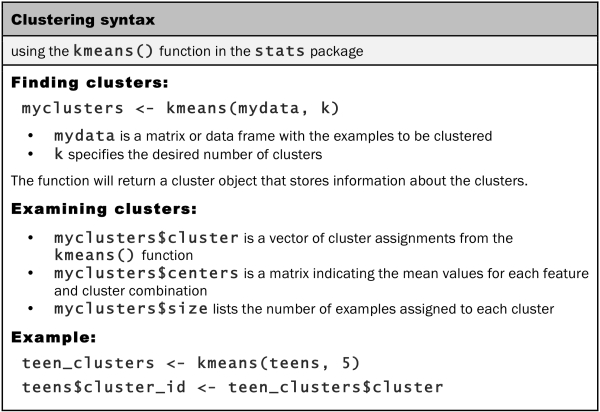
The kmeans() function requires a data frame containing only numeric data and a parameter specifying the desired number of clusters. If you have these two things ready, the actual process of building the model is simple. The trouble is that choosing the right combination of data and clusters can be a bit of an art; sometimes a great deal of trial and error is involved.
We'll start our cluster analysis by considering only the 36 features that represent the number of times various interests appeared on the teen SNS profiles. For convenience, let's make a data frame containing only these features:
> interests <- teens[5:40]
If you recall from Chapter 3, Lazy Learning – Classification Using Nearest Neighbors, a common practice employed prior to any analysis using distance calculations is to normalize or z-score standardize the features so that each utilizes the same range. By doing so, you can avoid a problem in which some features come to dominate solely because they have a larger range of values than the others.
The process of z-score standardization rescales features so that they have a mean of zero and a standard deviation of one. This transformation changes the interpretation of the data in a way that may be useful here. Specifically, if someone mentions football three times on their profile, without additional information, we have no idea whether this implies they like football more or less than their peers. On the other hand, if the z-score is three, we know that that they mentioned football many more times than the average teenager.
To apply the z-score standardization to the interests data frame, we can use the scale() function with lapply() as follows:
> interests_z <- as.data.frame(lapply(interests, scale))
Since lapply() returns a matrix, it must be coerced back to data frame form using the as.data.frame() function.
Our last decision involves deciding how many clusters to use for segmenting the data. If we use too many clusters, we may find them too specific to be useful; conversely, choosing too few may result in heterogeneous groupings. You should feel comfortable experimenting with the values of k. If you don't like the result, you can easily try another value and start over.
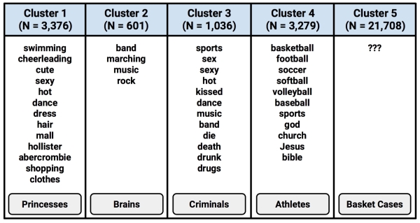
To help us predict the number of clusters in the data, I'll defer to one of my favorite films, The Breakfast Club, a coming-of-age comedy released in 1985 and directed by John Hughes. The teenage characters in this movie are identified in terms of five stereotypes: a brain, an athlete, a basket case, a princess, and a criminal. Given that these identities prevail throughout popular teen fiction, five seems like a reasonable starting point for k.
To use the k-means algorithm to divide the teenagers' interest data into five clusters, we use the kmeans() function on the interests data frame. Because the k-means algorithm utilizes random starting points, the set.seed() function is used to ensure that the results match the output in the examples that follow. If you recall from the previous chapters, this command initializes R's random number generator to a specific sequence. In the absence of this statement, the results will vary each time the k-means algorithm is run:
> set.seed(2345)
> teen_clusters <- kmeans(interests_z, 5)
The result of the k-means clustering process is a list named teen_clusters that stores the properties of each of the five clusters. Let's dig in and see how well the algorithm has divided the teens' interest data.
Evaluating clustering results can be somewhat subjective. Ultimately, the success or failure of the model hinges on whether the clusters are useful for their intended purpose. As the goal of this analysis was to identify clusters of teenagers with similar interests for marketing purposes, we will largely measure our success in qualitative terms. For other clustering applications, more quantitative measures of success may be needed.
One of the most basic ways to evaluate the utility of a set of clusters is to examine the number of examples falling in each of the groups. If the groups are too large or too small, they are not likely to be very useful. To obtain the size of the kmeans() clusters, use the teen_clusters$size component as follows:
> teen_clusters$size
[1]   871   600  5981  1034 21514
Here, we see the five clusters we requested. The smallest cluster has 600 teenagers (2 percent) while the largest cluster has 21,514 (72 percent). Although the large gap between the number of people in the largest and smallest clusters is slightly concerning, without examining these groups more carefully, we will not know whether or not this indicates a problem. It may be the case that the clusters' size disparity indicates something real, such as a big group of teens that share similar interests, or it may be a random fluke caused by the initial k-means cluster centers. We'll know more as we start to look at each cluster's homogeneity.
Tip
Sometimes, k-means may find extremely small clusters—occasionally, as small as a single point. This can happen if one of the initial cluster centers happens to fall on an outlier far from the rest of the data. It is not always clear whether to treat such small clusters as a true finding that represents a cluster of extreme cases, or a problem caused by random chance. If you encounter this issue, it may be worth re-running the k-means algorithm with a different random seed to see whether the small cluster is robust to different starting points.
For a more in-depth look at the clusters, we can examine the coordinates of the cluster centroids using the teen_clusters$centers component, which is as follows for the first four interests:
> teen_clusters$centers
   basketball   football      soccer    softball
1  0.16001227  0.2364174  0.10385512  0.07232021
2 -0.09195886  0.0652625 -0.09932124 -0.01739428
3  0.52755083  0.4873480  0.29778605  0.37178877
4  0.34081039  0.3593965  0.12722250  0.16384661
5 -0.16695523 -0.1641499 -0.09033520 -0.11367669
The rows of the output (labeled 1 to 5) refer to the five clusters, while the numbers across each row indicate the cluster's average value for the interest listed at the top of the column. As the values are z-score standardized, positive values are above the overall mean level for all the teens and negative values are below the overall mean. For example, the third row has the highest value in the basketball column, which means that cluster 3 has the highest average interest in basketball among all the clusters.
By examining whether the clusters fall above or below the mean level for each interest category, we can begin to notice patterns that distinguish the clusters from each other. In practice, this involves printing the cluster centers and searching through them for any patterns or extreme values, much like a word search puzzle but with numbers. The following screenshot shows a highlighted pattern for each of the five clusters, for 19 of the 36 teen interests:

Given this subset of the interest data, we can already infer some characteristics of the clusters. Cluster 3 is substantially above the mean interest level on all the sports. This suggests that this may be a group of Athletes per The Breakfast Club stereotype. Cluster 1 includes the most mentions of "cheerleading," the word "hot," and is above the average level of football interest. Are these the so-called Princesses?
By continuing to examine the clusters in this way, it is possible to construct a table listing the dominant interests of each of the groups. In the following table, each cluster is shown with the features that most distinguish it from the other clusters, and The Breakfast Club identity that most accurately captures the group's characteristics.
Interestingly, Cluster 5 is distinguished by the fact that it is unexceptional; its members had lower-than-average levels of interest in every measured activity. It is also the single largest group in terms of the number of members. One potential explanation is that these users created a profile on the website but never posted any interests.
Tip
When sharing the results of a segmentation analysis, it is often helpful to apply informative labels that simplify and capture the essence of the groups such as The Breakfast Club typology applied here. The risk in adding such labels is that they can obscure the groups' nuances by stereotyping the group members. As such labels can bias our thinking, important patterns can be missed if labels are taken as the whole truth.
Given the table, a marketing executive would have a clear depiction of five types of teenage visitors to the social networking website. Based on these profiles, the executive could sell targeted advertising impressions to businesses with products relevant to one or more of the clusters. In the next section, we will see how the cluster labels can be applied back to the original population for such uses.
Because clustering creates new information, the performance of a clustering algorithm depends at least somewhat on both the quality of the clusters themselves as well as what is done with that information. In the preceding section, we already demonstrated that the five clusters provided useful and novel insights into the interests of teenagers. By that measure, the algorithm appears to be performing quite well. Therefore, we can now focus our effort on turning these insights into action.
We'll begin by applying the clusters back onto the full dataset. The teen_clusters object created by the kmeans() function includes a component named cluster that contains the cluster assignments for all 30,000 individuals in the sample. We can add this as a column on the teens data frame with the following command:
> teens$cluster <- teen_clusters$cluster
Given this new data, we can start to examine how the cluster assignment relates to individual characteristics. For example, here's the personal information for the first five teens in the SNS data:
> teens[1:5, c("cluster", "gender", "age", "friends")]
  cluster gender    age friends
1       5      M 18.982       7
2       3      F 18.801       0
3       5      M 18.335      69
4       5      F 18.875       0
5       4   <NA> 18.995      10
Using the aggregate() function, we can also look at the demographic characteristics of the clusters. The mean age does not vary much by cluster, which is not too surprising as these teen identities are often determined before high school. This is depicted as follows:
> aggregate(data = teens, age ~ cluster, mean)
  cluster      age
1       1 16.86497
2       2 17.39037
3       3 17.07656
4       4 17.11957
5       5 17.29849
On the other hand, there are some substantial differences in the proportion of females by cluster. This is a very interesting finding as we didn't use gender data to create the clusters, yet the clusters are still predictive of gender:
> aggregate(data = teens, female ~ cluster, mean)
  cluster    female
1       1 0.8381171
2       2 0.7250000
3       3 0.8378198
4       4 0.8027079
5       5 0.6994515
Recall that overall about 74 percent of the SNS users are female. Cluster 1, the so-called Princesses, is nearly 84 percent female, while Cluster 2 and Cluster 5 are only about 70 percent female. These disparities imply that there are differences in the interests that teen boys and girls discuss on their social networking pages.
Given our success in predicting gender, you might also suspect that the clusters are predictive of the number of friends the users have. This hypothesis seems to be supported by the data, which is as follows:
> aggregate(data = teens, friends ~ cluster, mean)
  cluster  friends
1       1 41.43054
2       2 32.57333
3       3 37.16185
4       4 30.50290
5       5 27.70052
On an average, Princesses have the most friends (41.4), followed by Athletes (37.2) and Brains (32.6). On the low end are Criminals (30.5) and Basket Cases (27.7). As with gender, the connection between a teen's number of friends and their predicted cluster is remarkable, given that we did not use the friendship data as an input to the clustering algorithm. Also interesting is the fact that the number of friends seems to be related to the stereotype of each clusters' high school popularity; the stereotypically popular groups tend to have more friends.
The association among group membership, gender, and number of friends suggests that the clusters can be useful predictors of behavior. Validating their predictive ability in this way may make the clusters an easier sell when they are pitched to the marketing team, ultimately improving the performance of the algorithm.