In this section, we will discuss how much training samples are needed according to the situational context and highlight some important aspects when preparing your annotations on the positive training samples.
Let's start by defining the principle of object categorization and its relation to training data, which can be seen in the following figure:
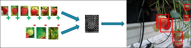
An example of positive and negative training data for an object model
The idea is that the algorithm takes a set of positive object instances, which contain the different presentations of the object you want to detect (this means object instances under different lighting conditions, different scales, different orientations, small shape changes, and so on) and a set of negative object instances, which contains everything that you do not want to detect with your model. Those are then smartly combined into an object model and used to detect new object instances in any given input image as seen in the figure above.
Many object detection algorithms depend heavily on large quantities of training data, or at least that is what is expected. This paradigm came to existence due to the academic research cases, mainly focusing on very challenging cases such as pedestrian and car detection. These are both object classes where a huge amount of intra-class variance exists, resulting in:
- A very large positive and negative training sample set, leading up to thousands and even millions of samples for each set.
- The removal of all information that pollutes the training set, rather than helping it, such as color information, and simply using feature information that is more robust to all this intra-class variation such as edge information and pixel intensity differences.
As a result, models were trained that successfully detect pedestrians and cars in about every possible situation, with the downside that training them required several weeks of processing.. However, when you look at more industrial specific cases, such as the picking of fruit from bins or the grabbing of objects from a conveyor belt, you can see that the amount of variance in objects and background is rather limited compared to these very challenging academic research cases. And this is a fact that we can use to our own advantage.
We know that the accuracy of the resulting object model is highly dependent on the training data used. In cases where your detector needs to work in all possible situations, supplying huge amounts of data seems reasonable. The complex learning algorithms will then decide which information is useful and which is not. However, in more confined cases, we could build object models by considering what our object model actually needs to do.
For example, the Facebook DeepFace application, used for detecting faces in every possible situation using the neural networks approach uses 4.4 million labeled faces.
We therefore suggest using only meaningful positive and negative training samples for your object model by following a set of simple rules:
- For the positive samples, only use natural occurring samples. There are many tools out there that create artificially rotated, translated, and skewed images to turn a small training set into a large training set. However, research has proven that the resulting detector is less performant than simply collecting positive object samples that cover the actual situation of your application. Better use a small set of decent high quality object samples, rather than using a large set of low quality non-representative samples for your case.
- For the negative samples, there are two possible approaches, but both start from the principle that you collect negative samples in the situation where your detector will be used, which is very different from the normal way of training object detects, where just a large set of random samples not containing the object are being used as negatives.
- Either point a camera at your scene and start grabbing random frames to sample negative windows from.
- Or use your positive images to your advantage. Cut out the actual object regions and make the pixels black. Use those masked images as negative training data. Keep in mind that in this case the ratio between background information and actual object occurring in the window needs to be large enough. If your images are filled with object instances, cutting them will result in a complete loss of relevant background information and thus reduce the discriminative power of your negative training set.
- Try to use a very small set of negative windows. If in your case only 4 or 5 background situations can occur, then there is no need to use 100 negative images. Just take those five specific cases and sample negative windows from them.
Efficiently collecting data in this way ensures that you will end up with a very robust model for your specific application! However, keep in mind that this also has some consequences. The resulting model will not be robust towards different situations than the ones trained for. However, the benefit in training time and the reduced need of training samples completely outweighs this downside.
Note
Software for negative sample generation based on OpenCV 3 can be found at https://github.com/OpenCVBlueprints/OpenCVBlueprints/tree/master/chapter_5/source_code/generate_negatives/.
You can use the negative sample generation software to generate samples like you can see in the following figure, where object annotations of strawberries are removed and replaced by black pixels.
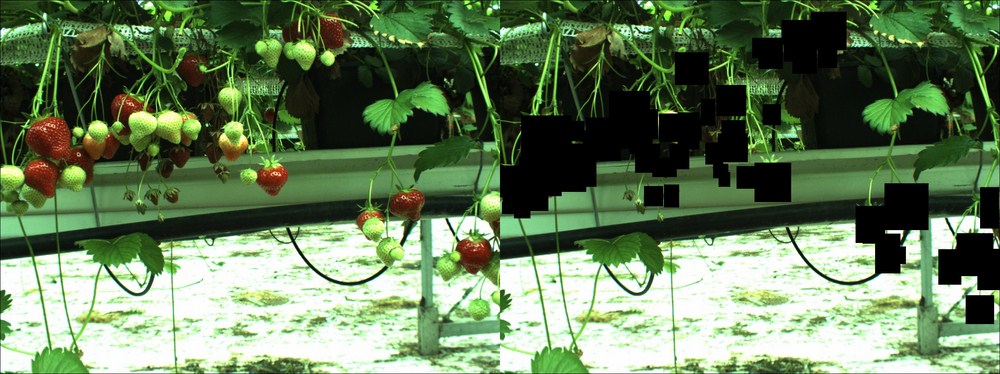
An example of the output of the negative image generation tool, where annotations are cut out and replaced by black pixels
As you can see, the ratio between the object pixels and the background pixels is still large enough in order to ensure that the model will not train his background purely based on those black pixel regions. Keep in mind that avoiding the approach of using these black pixelated images, by simply collecting negative images, is always better. However, many companies forget this important part of data collection and just end up without a negative data set meaningful for the application. Several tests I performed proved that using a negative dataset from random frames from your application have a more discriminative negative power than black pixels cutout based images.
When preparing your positive data samples, it is important to put some time in your annotations, which are the actual locations of your object instances inside the larger images. Without decent annotations, you will never be able to create decent object detectors. There are many tools out there for annotation, but I have made one for you based on OpenCV 3, which allows you to quickly loop over images and put annotations on top of them.
Note
Software for object annotation based on OpenCV 3 can be found at https://github.com/OpenCVBlueprints/OpenCVBlueprints/tree/master/chapter_5/source_code/object_annotation/.
The OpenCV team was kind enough to also integrate this tool into the main repository under the apps section. This means that if you build and install the OpenCV apps during installation, that the tool is also accessible by using the following command:
/opencv_annotation -images <folder location> -annotations <output file>
Using the software is quite straightforward:
- Start by running the CMAKE script inside the GitHub folder of the specific project. After running CMAKE, the software will be accessible through an executable. The same approach applies for every piece of software in this chapter. Running the CMAKE interface is quite straightforward:
cmakemake
./object_annotation -images <folder location> -annotations <output file>
- This will result in an executable that needs some input parameters, being the location of the positive image files and the output detection file.
- First, parse the content of your positive image folder to a file (by using the supplied
folder_listingsoftware inside the object annotation folder), and then follow this by executing the annotation command:./folder_listing –folder <folder> -images <images.txt> - The folder listing tool should generate a file, which looks exactly like this:
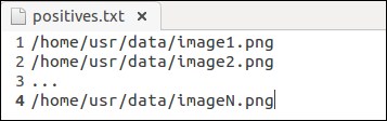
A sample positive samples file generated by the folder listing tool
- Now, fire up the annotation tool with the following command:
./object_annotation –images <images.txt> -annotations <annotations.txt> - This will fire up the software and give you the first image in a window, ready to apply annotations, as shown in the following figure:
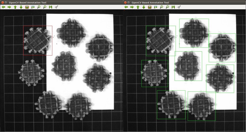
A sample of the object annotation tool
- You can start by selecting the top-left corner of the object, then moving the mouse until you reach the bottom right corner of the object, which can be seen in the left part of the preceding figure. However, the software allows you to start your annotation from each possible corner. If you are unhappy with the selection, then reapply this step, until the annotation suits your needs.
- Once you agree on the selected bounding box, press the button that confirms a selection, which is key C by default. This will confirm the annotation, change its color from red to green, and add it to the annotations file. Be sure only to accept an annotation if you are 100% sure of the selection.
- Repeat the preceding two steps for the same image until you have annotated every single object instance in the image, as seen in the right part of the preceding example image. Then press the button that saves the result and loads in the following image, which is the N key by default.
- Finally, you will end up with a file called
annotations.txt, which combines the location of the image files together with the ground truth locations of all object instances that occur inside the training images.
Note
If you want to adapt the buttons that need to be pressed for all the separate actions, then open up the object_annotation.cpp file and browse to line 100 and line 103. There you can adapt the ASCII values assigned to the button you want to use for the operation.
An overview of all ASCII codes assigned to your keyboard keys can be found at http://www.asciitable.com/.
The output from the software is a list of object detections in a *.txt file for each folder of positive image samples, which has a specific structure as seen in the following figure:
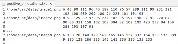
An example of an object annotation tool
It starts with the absolute file location of each image in the folder. There was a choice of not using relative paths since the file will then be fully dependent on the location where it is stored. However, if you know what you are doing, then using relative file locations in relation to the executable should work just fine. Using the absolute path makes it more universal and more failsafe. The file location is followed by the number of detections for that specific image, which allows us to know beforehand how many ground truth objects we can expect. For each of the objects, the (x, y) coordinates are stored to the top-left corner combined with the width and the height of the bounding box. This is continued for each image, which is each time a new line appears in the detection output file.
A second point of attention when processing positive training images containing object instances, is that you need to pay attention to the way you perform the actual placement of the bounding box of an object instance. A good and accurately annotated ground truth set will always give you a more reliable object model and will yield better test and accuracy results. Therefore, I suggest using the following points of attention when performing object annotation for your application:
- Make sure that the bounding box contains the complete object, but at the same time avoid as much background information as possible. The ratio of object information compared to background information should always be larger than 80%. Otherwise, the background could yield enough features to train your model on and the end result will be your detector model focusing on the wrong image information.
- Viola and Jones suggests using squared annotations, based on a 24x24 pixel model, because it fits the shape of a face. However, this is not mandatory! If your object class is more rectangular like, then do annotate rectangular bounding boxes instead of squares. It is observed that people tend to push rectangular shaped objects in a square model size, and then wonder why it is not working correctly. Take, for example, the case of a pencil detector, where the model dimensions will be more like 10x70 pixels, which is in relation to the actual pencil dimensions.
- Try doing concise batches of images. It is better to restart the application 10 times, than to have a system crash when you are about to finish a set of 1,000 images with corresponding annotations. If somehow, the software or your computer fails it ensures that you only need to redo a small set.
Before the OpenCV 3 software allows you to train a cascade classifier object model, you will need to push your data into an OpenCV specific data vector format. This can be done by using the provided sample creation tool of OpenCV.
Note
The sample creation tool can be found at https://github.com/Itseez/opencv/tree/master/apps/createsamples/ and should be built automatically if OpenCV was installed correctly, which makes it usable through the opencv_createsamples command.
Creating the sample vector is quite easy and straightforward by applying the following instruction from the command line interface:
./opencv_createsamples –info annotations.txt –vec images.vec –bg negatives.txt –num amountSamples –w model_width –h model_height
This seems quite straightforward, but it is very important to make no errors in this step of the setup and that you carefully select all parameters if you want a model that will actually be able to detect something. Let's discuss the parameters and instruct where to focus on:
-info: Add here the annotation file that was created using the object annotation software. Make sure that the format is correct, that there is no empty line at the bottom of the file and that the coordinates fall inside the complete image region. This annotation file should only contain positive image samples and no negative image samples as some online tutorials suggest. This would train your model to recognize negative samples as positives, which is not what we desire.-vec: This is the data format OpenCV will use to store all the image information and is the file that you created using the create samples software provided by OpenCV itself.-num: This is the actual number of annotations that you have inside the vector file over all the images presented to the algorithm. If you have no idea anymore how many objects you have actually annotated, then run the annotation counter software supplied.Note
The sample counting tool can be found at https://github.com/OpenCVBlueprints/OpenCVBlueprints/tree/master/chapter_5/source_code/count_samples/ and can be executed by the following command:
./count_samples -file <annotations.txt>
-wand-h: These are the two parameters that specify the final model dimensions. Keep in mind that these dimensions will immediately define the smallest object that you will be able to detect. Keep the size of the actual model therefore smaller than the smallest object you want to detect in your test images. Take, for example, the Viola and Jones face detector, which was trained on samples of 24x24 pixels, and will never be able to detect faces of 20x20 pixels.
When looking to the OpenCV 3 documentation on the "create samples" tool, you will see a wide range of extra options. These are used to apply artificial rotation, translation, and skew to the object samples in order to create a large training dataset from a limited set of training samples. This only works well when applying it to objects on a clean single color background, which can be marked and passed as the transparency color. Therefore, we suggest not to use these parameters in real-world applications and provide enough training data yourself using all the rules defined in the previous section.
Tip
If you have created a working classifier with, for example, 24x24 pixel dimensions and you still want to detect smaller objects, then a solution could be to upscale your images before applying the detector. However, keep in mind that if your actual object is, for example, 10x10 pixels, then upscaling that much will introduce tons of artifacts, which will render your model detection capabilities useless.
A last point of attention is how you can decide which is an effective model size for your purpose. On the one hand, you do not want it to be too large so that you can detect small object instances, on the other hand, you want enough pixel information so that separable features can be found.
Basically, what this software does is it takes an annotation file and processes the dimensions of all your object annotations. It then returns an average width and height of your object instances. You then need to apply a scaling factor to assign the dimensions of the smallest detectable object.
For example:
- Take a set of annotated apples in an orchard. You got a set of annotated apple tree images of which the annotations are stored in the apple annotation file.
- Pass the apple annotation file to the software snippet which returns you the average apple width and apple height. For now, we suppose that the dimensions for [waverage haverage] are [60 60].
- If we would use those [60 60] dimensions, then we would have a model that can only detect apples equal and larger to that size. However, moving away from the tree will result in not a single apple being detected anymore, since the apples will become smaller in size.
- Therefore, I suggest reducing the dimensions of the model to, for example, [30 30]. This will result in a model that still has enough pixel information to be robust enough and it will be able to detect up to half the apples of the training apples size.
- Generally speaking, the rule of thumb can be to take half the size of the average dimensions of the annotated data and ensure that your largest dimension is not bigger than 100 pixels. This last guideline is to ensure that training your model will not increase exponentially in time due to the large model size. If your largest dimension is still over 100 pixels, then just keep halving the dimensions until you go below this threshold.
You have now prepared your positive training set. The last thing you should do is create a folder with the negative images, from which you will sample the negative windows randomly, and apply the folder listing functionality to it. This will result in a negative data referral file that will be used by the training interface.