
Before we jump into the code, let's take an overview of the algorithm. There are four key components.
- The first is the pinhole camera model. We try and approximate real world positions to pixels using this matrix.
- The second is the camera motion estimate. We need to use data from the gyroscope to figure out the orientation of the phone at any given moment.
- The third is the rolling shutter computation. We need to specify the direction of the rolling shutter and estimate the duration of the rolling shutter.
- The fourth is the image warping expression. Using all the information from the previous calculations, we need to generate a new image so that it becomes stable.
We use the standard pinhole camera model. This model is used in several algorithms and is a good approximation of an actual camera.
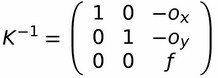
There are three unknowns. The o variables indicate the origin of the camera axis in the image plane (these can be assumed to be 0). The two 1s in the matrix indicate the aspect ratio of the pixels (we're assuming square pixels). The f indicates the focal length of the lens. We're assuming the focal length is the same in both horizontal and vertical directions.
Using this model, we can see that:
Here, X is the point in the real world. There is also an unknown scaling factor, q, present.
K is the intrinsic matrix and x is the point on the image.
We can assume that the world origin is the same as the camera origin. Then, the motion of the camera can be described in terms of the orientation of the camera. Thus, at any given time t:
The rotation matrix R can be calculated by integrating the angular velocity of the camera (obtained from the gyroscope).
Here, ωd is the gyroscope drift and td is the delay between the gyroscope and frame timestamps. These are unknowns as well; we need a mechanism to calculate them.
When you click a picture, the common assumption is that the entire image is captured in one go. This is indeed the case for images captured with CCD sensors (which were prevalent a while back). With the commercialization of CMOS image sensors, this is no longer the case. Some CMOS sensors support a global shutter too but, in this chapter, we'll assume the sensor has a rolling shutter.
Images are captured one row at a time—usually the first row is captured first, then the second row, and so on. There's a very slight delay between the consecutive rows of an image.
This leads to strange effects. This is very visible when we're correcting camera shake (for example if there's a lot of motion in the camera).
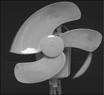
The fan blades are the same size; however due to the fast motion, the rolling shutter causes artifacts in the image recorded by the sensor.
To model the rolling shutter, we need to identify at what time a specific row was captured. This can be done as follows:
Here, ti is the time when the ith frame was captured, h is the height of the image frame, and ts is the duration of the rolling shutter, that is, the time it takes to scan from top to bottom. Assuming each row takes the same time, the yth row would take ts * y / h additional time to get scanned.
So far, we have the estimated camera motion and a model for correcting the rolling shutter. We'll combine both and identify a relationship across multiple frames:
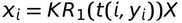 (for frame i with rotation configuration 1)
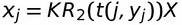 (for frame j with rotation configuration 2)
We can combine these two equations:
From here, we can calculate a warping matrix:
Now, the relationship between points xi and xj can be more succinctly described as:
This warp matrix simultaneously corrects both the video shake and the rolling shutter.
Now we can map the original video to an artificial camera that has smooth motion and a global shutter (no rolling shutter artifacts).
This artificial camera can be simulated by low-pass filtering the input camera's motion and setting the rolling shutter duration to zero. A low pass filter removes high frequency noise from the camera orientation. Thus, the artificial camera's motion will appear much smoother.
Ideally, this matrix can be calculated for each row in the image. However, in practice, subdividing the image into five subsections produces good results as well (with better performance).