
Once you have built a decent training samples dataset, which is ready to process, the time has arrived to fire up the cascade classifier training software of OpenCV 3, which uses the Viola and Jones cascade classifier framework to train your object detection model. The training itself is based on applying the boosting algorithm on either Haar wavelet features or Local Binary Pattern features. Several types of boosting are supported by the OpenCV interface, but for convenience, we use the frequently used AdaBoost interface.
Note
If you are interested in knowing all the technical details of the feature calculation, then have a look at the following papers which describe them in detail:
- HAAR: Papageorgiou, Oren and Poggio, "A general framework for object detection", International Conference on Computer Vision, 1998.
- LBP: T. Ojala, M. Pietikäinen, and D. Harwood (1994), "Performance evaluation of texture measures with classification based on Kullback discrimination of distributions", Proceedings of the 12th IAPR International Conference on Pattern Recognition (ICPR 1994), vol. 1, pp. 582 - 585.
This section will discuss several parts of the training process in more detail. It will first elaborate on how OpenCV runs its cascade classification process. Then, we will take a deeper look at all the training parameters provided and how they can influence the training process and accuracy of the resulting model. Finally, we will open up the model file and look in more detail at what we can find there.
It is important to pay attention when carefully selecting your training parameters. In this subsection, we will discuss the relevance of some of the training parameters used when training and suggest some settings for general testing purposes. The following subsection will then discuss the output and the quality of the resulting classifier.
First, start by downloading and compiling the cascade classifier training application which is needed for generating an object detection model using the Viola and Jones framework.
Note
The cascade classification training tool can be found at https://github.com/Itseez/opencv/tree/master/apps/traincascade/. If you build the OpenCV apps and installed them, then it will be directly accessible by executing the ./train_cascade command.
If you run the application without the parameters given, then you will get a print of all the arguments that the application can take. We will not discuss every single one of them, but focus on the most delicate ones that yield the most problems when training object models using the cascade classifier approach. We will give some guidelines as how to select correct values and where to watch your steps. You can see the output parameters from the cascade classifier training interface in the following figure:

The opencv_traincascade input parameters in OpenCV 3
-data: This parameter contains the folder where you will output your training results. Since the creation of folders is OS specific, OpenCV decided that they will let users handle the creation of the folder. If you do not make it in advance, training results will not be stored correctly. The folder will contain a set of XML files, one for the training parameters, one for each trained stage and finally a combined XML file containing the object model.-numPos: This is the amount of positive samples that will be used in training each stage of weak classifiers. Keep in mind that this number is not equal to the total amount of positive samples. The classifier training process (discussed in the next subtopic) is able to reject positive samples that are wrongfully classified by a certain stage limiting further stages to use that positive sample. A good guideline in selecting this parameter is to multiply the actual amount of positive samples, retrieved by the sample counter snippet, with a factor of 0.85.-numNeg: This is the amount of negative samples used at each stage. However, this is not the same as the amount of negative images that were supplied by the negative data. The training samples negative windows from these images in a sequential order at the model size dimensions. Choosing the right amount of negatives is highly dependent on your application.- If your application has close to no variation, then supplying a small number of windows could simply do the trick because they will contain most of the background variance.
- On the other hand, if the background variation is large, a huge number of samples would be needed to ensure that you train as much random background noise as possible into your model.
- A good start is taking a ratio between the number of positive and the number of negative samples equaling 0.5, so double the amount of negative versus positive windows.
- Keep in mind that each negative window that is classified correctly at an early stage will be discarded for training in the next stage since it cannot add any extra value to the training process. Therefore, you must be sure that enough unique windows can be grabbed from the negative images. For example, if a model uses 500 negatives at each stage and 100% of those negatives get correctly classified at each stage, then training a model of 20 stages will need 10,000 unique negative samples! Considering that the sequential grabbing of samples does not ensure uniqueness, due to the limited pixel wise movement, this amount can grow drastically.
-numStages: This is the amount of weak classifier stages, which is highly dependent on the complexity of the application.- The more stages, the longer the training process will take since it becomes harder at each stage to find enough training windows and to find features that correctly separate the data. Moreover, the training time increases in an exponential manner when adding stages.
- Therefore, I suggest looking at the reported acceptance ratio that is outputted at each training stage. Once this reaches values of 10^(-5), you can conclude that your model will have reached the best descriptive and generalizing power it could get, according to the training data provided.
- Avoid training it to levels of 10^(-5) or lower to avoid overtraining your cascade on your training data. Of course, depending on the amount of training data supplied, the amount of stages to reach this level can differ a lot.
-bg: This refers to the location of the text file that contains the locations of the negative training images, also called the negative samples description file.-vec: This refers to the location of the training data vector that was generated in the previous step using the create_samples application, which is built-in to the OpenCV 3 software.-precalcValBufSizeand-precalcIdxBufSize: These parameters assign the amount of memory used to calculate all features and the corresponding weak classifiers from the training data. If you have enough RAM memory available, increase these values to 2048 MB or 4096 MB, which will speed up the precalculation time for the features drastically.-featureType: Here, you can choose which kind of features are used for creating the weak classifiers.- HAAR wavelets are reported to give higher accuracy models.
- However, consider training test classifiers with the LBP parameter. It decreases training time of an equal sized model drastically due to the integer calculations instead of the floating point calculations.
-minHitRate: This is the threshold that defines how much of your positive samples can be misclassified as negatives at each stage. The default value is 0.995, which is already quite high. The training algorithm will select its stage threshold so that this value can be reached.- Making it 0.999, as many people do, is simply impossible and will make your training stop probably after the first stage. It means that only 1 out of 1,000 samples can be wrongly classified over a complete stage.
- If you have very challenging data, then lowering this, for example, to 0.990 could be a good start to ensure that the training actually ends up with a useful model.
-maxFalseAlarmRate: This is the threshold that defines how much of your negative samples need to be classified as negatives before the boosting process should stop adding weak classifiers to the current stage. The default value is 0.5 and ensures that a stage of weak classifier will only do slightly better than random guessing on the negative samples. Increasing this value too much could lead to a single stage that already filters out most of your given windows, resulting in a very slow model at detection time due to the vast amount of features that need to be validated for each window. This will simply remove the large advantage of the concept of early window rejection.
The parameters discussed earlier are the most important ones to dig into when trying to train a successful classifier. Once this works, you can increase the performance of your classifier even more, by looking at the way boosting forms its weak classifiers. This can be adapted by the -maxDepth and -maxWeakCount parameters. However, for most cases, using stump weak classifiers (single layer decision trees) on single features is the best way to start, ensuring that single stage evaluation is not too complex and thus fast at detection time.
Once you select the correct training parameters, you can start the cascade classifier training process, which will build your cascade classifier object detection model. In order to fully understand the cascade classification process that builds up your object model, it is important to know how OpenCV does its training of the object model, based on the boosting process.
Before we do this, we will have a quick look at the outline of the boosting principle in general.
The idea behind boosting is that you have a very large pool of features that can be shaped into classifiers. Using all those features for a single classifier would mean that every single window in your test image will need to be processed for all these features, which will take a very long time and make your detection slow, especially if you consider how many negative windows are available in a test image. To avoid this, and to reject as many negative windows as fast as possible, boosting selects the features that are best at separating the positive and negative data and combines them into classifiers, until the classifier does a bit better than random guessing on the negative samples. This first step is called a weak classifier. Boosting repeats this process until the combination of all these weak classifiers reach the desired accuracy of the algorithm. The combination is called the strong classifier. The main advantage of this process is that tons of negative samples will already be discarded by the few early stages, with only evaluating a small set of features, thus decreasing detection time a lot.
We will now try to explain the complete process using the output generated by the cascade training software embedded in OpenCV 3. The following figure illustrates how a strong cascade classifier is built from a set of stages of weak classifiers.

A combination of weak classifier stages and early rejection of misclassified windows resulting in the famous cascade structure
The cascade classifier training process follows an iterative process to train subsequent stages of weak classifiers (1…N). Each stage consists of a set of weak classifiers, until the criteria for that specific stage have been reached. The following steps are an overview of what is happening at training each stage in OpenCV 3, according to the input parameters given and the training data provided. If you are interested in more specific details of each subsequent step, then do read the research paper of Viola and Jones (you can have a look at the citation on the first page of this chapter) on cascade classifiers. All steps described here are subsequently repeated for each stage until the desired accuracy for the strong classifier is reached. The following figure shows how such a stage output looks like:

An example output of a classifier stage training
You will notice that the first thing the training does is grabbing training samples for the current stage—first the positive samples from the data vector you supplied, and then the random negative window samples from the negative images that you supplied. This will be outputted for both steps as:
POS:number_pos_samples_grabbed:total_number_pos_samples_needed NEG:number_neg_samples_grabbed:acceptanceRatioAchieved
If no positive samples can be found anymore, an error will be generated and training will be stopped. The total number of samples needed will increase once you start discarding positives that are no longer useful. The grabbing of the negatives for the current stage can take much longer than the positive sample grabbing since all windows that are correctly classified by the previous stages are discarded and new ones are searched. The deeper you go into the amount of stages, the harder this gets. As long as the number of samples grabbed keeps increasing (and yes, this can be very slow, so be patient), your application is still running. If no more negatives are found, the application will end training and you will need to lower the amount of negatives for each stage or add extra negative images.
The acceptance ratio that is achieved by the previous stage is reported after the grabbing of the negative windows. This value indicates whether the model trained until now is strong enough for your detection purposes or not!
Once we have both positive and negative window-sized samples, the precalculation will calculate every single feature that is possible within the window size and apply it for each training sample. This can take some time according to the size of your model and according to the amount of training samples, especially when knowing that a model of 24x24 pixels can yield more than 16,000 features. As suggested earlier, assigning more memory can help out here or you could decide on selecting LBP features, of which the calculation is rather fast compared to HAAR features.
All features are calculated on the integral image representation of the original input window. This is done in order to speed up the calculation of the features. The paper by Viola and Jones explains in detail why this integral image representation is used.
The features calculated are dumped into a large feature pool from which the boosting process can select the features needed to train the weak classifiers that will be used within each stage.
Now, the cascade classifier training is ready for the actual boosting process. This happens in several small steps:
- Every possible weak classifier inside the feature pool is being calculated. Since we use stumps, which are basically weak classifiers based on single feature to create a decision tree, there are as many weak classifiers as features. If you prefer, you can decide to train actual decision trees with a predefined maximum depth, but this goes outside of the scope of this chapter.
- Each weak classifier is trained in order to minimize the misclassification rate on the training samples. For example, when using Real AdaBoost as a boosting technique, the Gini index is minimized.
- The weak classifier with the lowest misclassification rate is added as the next weak classifier to the current stage.
- Based on the weak classifiers that are already added to the stage, the algorithm calculates the overall stage threshold, which is set so that the desired hit rate is guaranteed.
- Now, the weights of the samples are adapted based on their classification in the last iteration, which will yield a new set of weak classifiers in the next iteration, and thus the whole process can start again.
- During the combination of the weak classifiers inside a single stage, which is visualized in the training output, the boosting process makes sure that:
- The overall stage threshold does not drop below the minimum hit rate that was selected by the training parameters.
- The false alarm rate on the negative samples decreases compared to the previous stage.
- This process continues until:
- The false acceptance ratio on the negative samples is lower than the maximum false alarm rate set. The process then simply starts training a new stage of weak classifiers for the detection model.
- The required stage false alarm rate is reached, which is
maxFalseAlarmRate^#stages. This will yield an end to the model training since the model satisfies our requirements and better results cannot be achieved anymore. This will not happen often, since this value drops rather quickly, and after several stages, this would mean that you correctly classify more than 99% of your positive and negative samples all together. - The hit rate drops below the stage specific minimal hit rate, which is the
minHitRate^#stages. At this stage, too many positives get wrongly classified and the maximum performance for your model is reached.
After training each stage, the stage specific details about the weak classifiers and the thresholds are stored in the data folder, in a separate XML file. If the desired number of stages has been reached, then these subfiles are combined into a single cascade XML file.
However, the fact that every stage is stored separately means that you can stop the training at any time and create an in-between object detection model, by simply restarting the training command, but changing the -numStages parameter to the stage value on which you want to check the model's performance. This is ideal when you want to perform an evaluation on a validation set to ensure that your model does not start overfitting on the training data!
It has been observed that many users of the cascade classifier algorithm embedded in OpenCV 3 do not know the meaning of the inner construction of the object model which is stored in the XML files, which sometimes leads to wrong perceptions of the algorithm. This subsection will explain each internal part of the trained object models. We will discuss a model based on stump-typed weak classifiers, but the idea is practically the same for any other type of weak classifiers inside a stage, such as decision trees. The biggest difference is that the weight calculation inside the model gets more complex as compared to when using stump features. As to the weak classifiers structure inside each stage, this will be discussed for both HAAR- and LBP-based features since these are the two most used features inside OpenCV for training cascade classifiers.
The first part of each XML stored model describes the parameters that specify the characteristics of the model itself and some of the important training parameters. Subsequently, we can find the type of training that is used, which is limited to boosting for now, and the type of features used for building the weak classifiers. We also have the width and height of the object model that will be trained, the parameters of the boosting process, which include the type of boosting used, the selected minimum hit ratio, and the selected maximum false acceptance rate. It also contains information about how the weak classifier stages are built, in our case as a combination of one feature deep trees, called stumps, with a maximum of 100 weak classifiers on a single stage. For the HAAR wavelet based model, we can then see which features are used, being only the basic upright features or the combined rotated 45-degree set.
After the training-specific parameters, it starts to get interesting. Here, we find more information about the actual structure of the cascade classifier object model. The amount of stages is described, and then iteratively the model sums up the training results and thresholds for each separate stage which were generated by the boosting process. The basic structure of an object model can be seen here:
<stages>
    <_>
        <maxWeakCount></maxWeakCount>
        <stageThreshold</stageThreshold>
        <weakClassifiers>
            <!-- tree 0 -->
            <_>
                <internalNodes></internalNodes>
                <leafValues></leafValues></_>
            <!-- tree 1 -->
            <_>
                <internalNodes></internalNodes>
                <leafValues></leafValues></_>
            <!-- tree 2 -->
            … … …
    <!-- stage 1 -->
    … … …
</stages>
<features>
    … … …
</features>
We start with an empty iteration tag for each stage. At each stage the number of weak classifiers that were used are defined, which in our case shows how many single layer decision trees (stumps) were used inside the stage. The stage threshold defines the threshold on the final stage score for a window. This is generated by scoring the window with each weak classifier and then summing and weighing the results for the complete stage. For each single weak classifier, we collect the internal structure, based on the decision nodes and layers used. The values present are the boosting values used for creating the decision tree and the leaf values, which are used to score a window that is evaluated by the weak classifier.
The specifics for the internal node structure are different for HAAR wavelets and -based features. The storage of the leaf scores is equal. The values of the internal nodes, however, specify the relation to the bottom part of the code, which contains the actual features area, and which are also different for both the HAAR and the LBP approach. The difference between both techniques can be seen in the following sections, grabbing for both models the first tree of the first stage and a part of the feature set.
The following are two code snippets from the HAAR wavelet feature-based model, containing the internal node structure and the features structure:
<internalNodes>
0 -1 445 -1.4772760681807995e-02
</internalNodes>
… … …
<_>
    <rects>
        <_>23 10 1 3 -1.</_>
        <_>23 11 1 1 3.</_>
    </rects>
    <tilted>0</tilted>
</_>
For the internal nodes, there are four values present at each node:
- Node left and node right: These values indicate that we have a stump with two leafs.
- The node feature index: This points the index of the feature used at this node according to its position inside the features list of that model.
- The node threshold: This is the threshold that is set on the feature value for this weak classifier, which is learned from all the positive and negative samples in this stage of training. Since we are looking at models with stump based weak classifiers, this is also the stage threshold, which is set in the boosting process.
The features inside the HAAR-based model are described by a set of rectangles, which can be up to three rectangles, so as to calculate every possible feature from a window. Then, there is a value indicating if the feature itself is tilted over 45 degrees or not. For each rectangle, which is a partial feature value, we have:
- The location of the rectangle, which is defined by upper-left corner x and y coordinates and the width and height of the rectangle.
- The weight for that specific partial feature. These weights are used to combine both partial feature rectangles into a predefined feature. These weights allow us to represent each feature with less rectangles than is actually necessary. An example of this can be seen in the following figure:

A three rectangle feature can be represented by a two rectangle weighted combination reducing the need of an extra area calculation
The feature sum is finally calculated by first summing all values of the pixels inside the rectangle and then multiplying it with the weight factor. Finally, those weighted sums are combined together to yield as a final feature value. Keep in mind that all the coordinates retrieved for a single feature are in relation to the window/model size and not the complete image which is processed.
The following are two code snippets from the LBP feature-based model, containing the internal node structure and the features structure:
<internalNodes>
0 -1 46 -67130709 -21569 -1426120013 -1275125205 -21585
-16385 587145899 -24005
</internalNodes>
… … …
<_>
    <rect>0 0 3 5</rect>
</_>
For the internal nodes, there are 11 values present at each node:
- Node left and node right: These values indicate that we have a stump with two leafs, which is identical to the HAAR-based model. If a more complex tree structure is used, these values will expand.
- The node feature index: This points to the index of the feature used at this node according to its position inside the features list of that model.
- Eight 32-bit values: These values together in the combined form of a 256-bit LUT are calculated by comparing all subrectangle regions to the center subrectangle, as illustrated in the following figure, and which is used as a threshold to yield 1 or 0 as an outcome for the descriptor of the feature.
For the features inside the LBP based model, we have the dimensions (x, y, w, h) of a single subrectangle region (the top-left subrectangle) out of the nine that are needed for the LBP feature to be evaluated, as seen here:

An example of a LBP feature-based on the single stored rectangle
However, there is nothing better than seeing your trained object model visualized on the object you have been training for. Therefore, I programmed a code snippet that takes a model and a base image and visualizes the complete model detection process on top of it.
Note
The software for visualizing Haar wavelet or LBP models can be found at https://github.com/OpenCVBlueprints/OpenCVBlueprints/tree/master/chapter_5/source_code/visualize_models/.
The software takes in several input arguments, such as the model location, the image where the visualization needs to happen, and the output folder where the results need to be stored. However, in order to use the software correctly, there are some points of attention:
- The model needs to be HAAR wavelet or LBP feature based. Deleted because this functionality is no longer supported in OpenCV 3.
- You need to supply an image that is an actual model detection for visualization purposes and resize it to the model scale or a positive training sample from the training data. This is to ensure that a feature of your model is placed at the correct location.
- Inside the code, you can adapt the visualization scales, one being for the video output of your model and one for the images that represent the stages.
The following two figures illustrate the visualization result of the Haar wavelet and LBP feature based frontal face model respectively, both incorporated into the OpenCV 3 repository under the data folder. The reason for the low image resolution of the visualization is quite obvious. The training process happens on a model scale; therefore, I wanted to start from an image of that size to illustrate that specific details of an object get removed, while general specifics of the object class still occur to be able to differentiate classes.

A set of frames from the video visualization of the frontal face model for both Haar wavelet and Local Binary Pattern features
The visualizations for example also clearly show that an LBP model needs less features and thus less weak classifiers to separate the training data successfully, which yields a faster model at detection time.
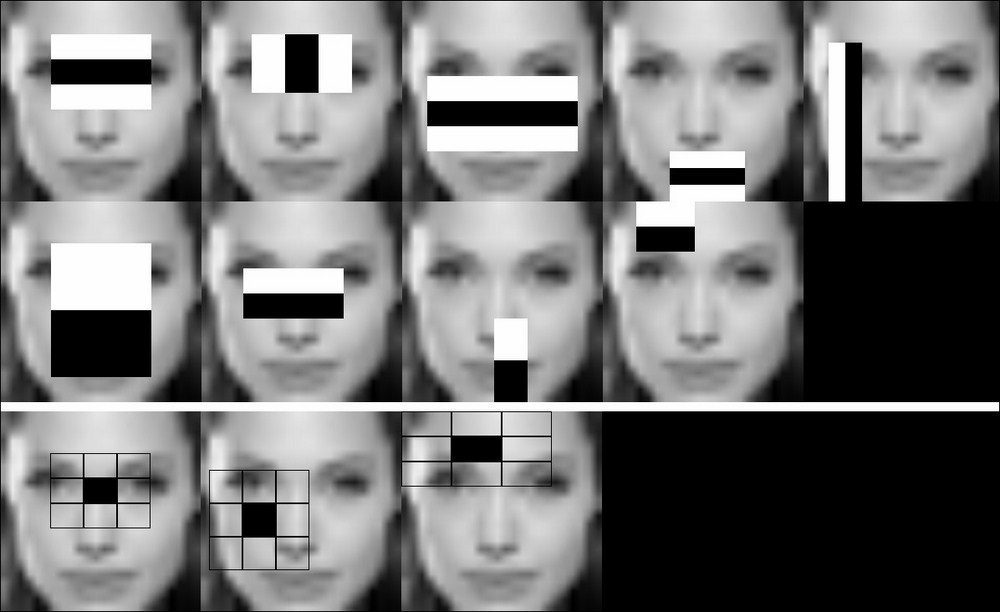
A visualization of the first stage of the frontal face model for both Haar wavelet and Local Binary Pattern features
Making sure that you get the absolute best model given your training, testing the data can be done by applying a cross validation approach, such as the leave-one-out approach. The idea behind this is that you combine both training and test set and vary the test set that you use from the larger set. With each random test set and training set, you build a separate model and you perform the evaluation using precision-recall, which is discussed further in this chapter. Finally, the model that provides the best result could be adopted as a final solution. Thus, it could mitigate the impact of an error due to a new instance that is not represented in the training set.