We are heading towards the end of this chapter, but before we end, I would like to address two small but still important topics. Let's start by discussing the evaluation of the performance of cascade classifier object detection models by using not only a visual check but by actually looking at how good our model performs over a larger dataset.
We will do this by using the concept of precision recall curves. They differ a bit from the more common ROC curves from the statistics field, which have the downside that they depend on true negative values, and with sliding windows applications, this value becomes so high that the true positive, false positive, and false negative values will disappear in relation to the true negatives. Precision-recall curves avoid this measurement and thus are better for creating an evaluation of our cascade classifier model.
Precision = TP / (TP + FP) and Recall = TP / (TP + FN) with a true positive (TP) being an annotation that is also found as detection, a false positive (FP) being a detection for which no annotation exist, and a false negative (FN) being an annotation for which no detection exists.
These values describe how good your model works for a certain threshold value. We use the certainty score as a threshold value. The precision defines how much of the found detections are actual objects, while the recall defines how many of the objects that are in the image are actually found.
Note
Software for creating PR curves over a varying threshold can be found at https://github.com/OpenCVBlueprints/OpenCVBlueprints/tree/master/chapter_5/source_code/precision_recall/.
The software requires several input elements:
- First of all, you need to collect a validation/test set that is independent of the training set because otherwise you will never be able to decide if your model was overfitted for a set of training data and thus worse for generalizing over a set of class instances.
- Secondly, you need an annotation file of the validation set, which can be seen as a ground truth of the validation set. This can be made with the object annotation software that is supplied with this chapter.
- Third, you need a detection file created with the detection software that also outputs the score, in order to be able to vary over those retrieved scores. Also, ensure that the nonmaxima suppression is only set at 1 so that detections on the same location get merged but none of the detections get rejected.
When running the software on such a validation set, you will receive a precision recall result file as shown here. Combined with a precision recall coordinate for each threshold step, you will also receive the threshold itself, so that you could select the most ideal working point for your application in the precision recall curve and then find the threshold needed for that!
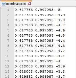
Precision recall results for a self trained cascade classifier object model
This output can then be visualized by software packages such as MATLAB (http://nl.mathworks.com/products/matlab/) or Octave (http://www.gnu.org/software/octave/), which have better support for graph generation than OpenCV. The result from the preceding file can be seen in the following figure. A MATLAB sample script for generating those visualizations is supplied together with the precision recall software.
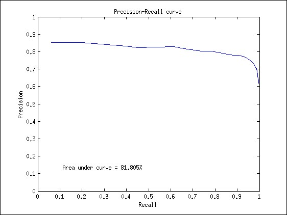
Precision recall results on a graph
Looking at the graph, we see that both precision and recall have a scale of [0 1]. The most ideal point in the graph would be the upper-right corner (precision=1/recall=1), which would mean that all objects in the image are found and that no false positive detections are found. So basically, the closer the slope of your graph goes towards the upper right corner, the better your detector will be.
In order to add a value of accuracy to a certain curve of the precision recall graph (when comparing models with different parameters), the computer vision research community uses the principle of the area under the curve (AUC), expressed in a percentage, which can also be seen in the generated graph. Again, getting an AUC of 100% would mean that you have developed the ideal object detector.
To be able to reconstruct the experiments done in the discussion about GPU usage, you will need to have an NVIDIA GPU, which is compatible with the OpenCV CUDA module. Furthermore, you will need to rebuild OpenCV with different configurations (which I will highlight later) to get the exact same output.
The tests from my end were done with a Dell Precision T7610 computer containing an Intel Xeon(R) CPU that has two processors, each supporting 12 cores and 32 GB of RAM memory. As GPU interface, I am using an NVIDIA Quadro K2000 with 1 GB of dedicated on-board memory.
Similar results can be achieved with a non-NVIDIA GPU through OpenCL and the newly introduced T-API in OpenCV 3. However, since this technique is fairly new and still not bug free, we will stick to the CUDA interface.
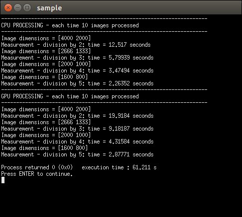
OpenCV 3 contains a GPU implementation of the cascade classifier detection system, which can be found under the CUDA module in. This interface could help to increase the performance when processing larger images. An example of that can be seen in the following figure:
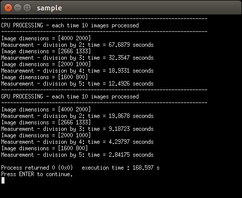
CPU-GPU comparison without using any CPU optimizations
Note
These results were obtained by using the software that can be retrieved from https://github.com/OpenCVBlueprints/OpenCVBlueprints/tree/master/chapter_5/source_code/CPU_GPU_comparison/.
For achieving this result, I built OpenCV without any CPU optimization and CUDA support. For this, you will need to disable several CMAKE flags, thus disabling the following packages: IPP, TBB, SSE, SSE2, SSE3, SSE4, OPENCL, and PTHREAD. In order to avoid any bias from a single image being loaded at a moment that the CPU is doing something in the background, I processed the image 10 times in a row.
The original input image has a size of 8000x4000 pixels, but after some testing, it seemed that the detectMultiScale function on GPU would require memory larger than the dedicated 1 GB. Therefore, we only run tests starting from having the image size as 4000*2000 pixels. It is clear that, when processing images on a single core CPU, the GPU interface is way more efficient, even if you take into account that at each run, it needs to push data from memory to the GPU and get it back. We still get a speedup of about 4-6 times.
However, the GPU implementation is not always the best way to go, as we will prove by a second test. Let's start by summing up some reasons why the GPU could be a bad idea:
- If your image resolution is small, then it is possible that the time needed to initialize the GPU, parse the data towards the GPU, process the data, and grab it back to memory will be the bottleneck in your application and will actually take longer than simply processing it on the CPU. In this case, it is better to use a CPU-based implementation of the detection software.
- The GPU implementation does not provide the ability to return the stage weights and thus creating a precision recall curve based on the GPU optimized function will be difficult.
- The preceding case was tested with a single core CPU without any optimizations, which is actually a bad reference nowadays. OpenCV has been putting huge efforts into making their algorithms run efficiently on CPU with tons of optimizations. In this case, it is not for granted that a GPU with the data transfer bottleneck will still run faster.
To prove the fact that a GPU implementation can be worse than a CPU implementation, we built OpenCV with the following freely available optimization parameters: IPP (free compact set provided by OpenCV), TBB, SSE2, SSE3, SSE4 (SSE instructions selected automatically by the CMAKE script for my system), pthread (for using parallel for loop structures), and of course, with the CUDA interface.
We will then run the same software test again, as shown here.
CPU-GPU comparison with basic CPU optimizations provided by OpenCV 3.0
We will clearly see now that using the optimizations on my system yield a better result on CPU than on GPU. In this case, one would make a bad decision by only looking at the fact that he/she has a GPU available. Basically, this proves that you should always pay attention to how you will optimize your algorithm. Of course, this result is a bit biased, since a normal computer does not have 24 cores and 32 GB of RAM memory, but seeing that the performance of personal computers increase every day, it will not take long before everyone has access to these kind of setups.
I even took it one step further, by taking the original image of 8000*4000 pixels, which has no memory limits on my system for the CPU due to the 32 GB or RAM, and performed the software again on that single size. For the GPU, this meant that I had to break down the image into two parts and process those. Again, we processed 10 images in a row. The result can be seen in the following image:
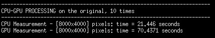
Comparison of an 8000x4000 pixel processed on GPU versus multicore CPU
As you can see, there is still a difference of the GPU interface taking about four times as long as the CPU interface, and thus in this case, it would be a very bad decision to select a GPU solution for the project, rather than a multicore CPU solution.