
In the preceding chapters, we covered some fundamental data structures and algorithms. The current chapter extends static algorithm (deterministic algorithm) concepts to randomized algorithms. Deterministic algorithms use polynomials of the size of the input, whereas random algorithms use random sources as input and make their own choices. The chapter will introduce the Las Vegas and the Monte Carlo randomized algorithms and their application using examples. The chapter will also introduce skip list and its extended version, randomized skip list, which uses randomization concepts to reduce the computation effort in an average case scenario. We will start with the fundamentals of programming, which can be used to reduce computational effort in intensive tasks. The current chapter will cover the concepts of dynamic programming and directed acyclic graphs (DAGs). The current chapter will cover following topics:
- Dynamic programming
- The knapsack problem
- All-pairs shortest paths
- Randomized algorithms
- Randomized algorithms for finding large values
- Skip lists
Dynamic programming can be defined as an approach that uses a recurrent formula (breaking a problem into a subproblem) to solve any complex problem. A sub-solution of any problem is reconstructed using the previous state solution. Dynamic programming-based approaches are able to achieve a polynomial complexity for solving problems, and assure faster computation than other classical approaches, such as brute force algorithms. Before we get into dynamic programming, let's cover the basics of DAG, as it will help with implementation of dynamic programming. DAGs are directed acyclic topological graphs, which are defined by a number of vertices and edges such that every edge is directed from earlier to later in the sequence. An example of a DAG is shown in Figure 9.1:

Figure 9.1: An example of DAG
Let's assume that the vertices represent cities and edges represent the path to be followed to reach a particular city. The objective is to determine the shortest path to node D from root node A in the preceding figure. This can be represented as follows:
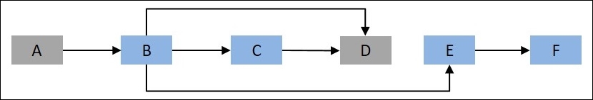
Figure 9.2: Another representation of Figure 9.1, with the objective to reach node D from the root node, A
Let d(i,j) represent the distance from the ith vertex to the jth vertex, so in the example, d(A, B) represents the distance from node A to node B. Also, mdist(k) represents the shortest distance to the kth vertex. The minimum distance to D can be written as follows:
Shortest_Distance(A, D) = min{ mdist(B)+ d(B, D), mdist(D)+d(C, D)}
Similarly, mdist(k) can be further broken down into subproblems. DAG is implicit in dynamic programming, where each vertex acts a subproblem and an edge represents the dependency between subproblems. The approach of dynamic programming is very different from recursion. Let's consider an example for writing a function to calculate the nth Fibonacci series. The Fibonacci series is a sequence of integers such that every number is a sum of the preceding two numbers: {1, 1, 2, 3, 5, 8, ...}. The function for evaluating the nth Fibonacci number can be written using recursion in R, as shown here:
nfib<-function(n){
  assertthat::assert_that(n>0) & assertthat::assert_that(n<50)
  if(n==1 || n==2) return(1)
  val<- nfib(n-1) + nfib(n-2)
  return(val)
}
Let's look at how the recursive approach processes the computation of the nth Fibonacci number. Figure 9.3 shows how the preceding recursive function nfibonacci will evaluate the sixth Fibonacci number:

Figure 9.3: Number of times the nfibonacci function is called to calculate the sixth Fibonacci number
From Figure 9.3 it is evident that in the recursive approach, the lower values are computed multiple times thus making the algorithm sub-optimal; however, computational time increases exponentially due to repeated computation of the same values, as shown in Figure 9.4:

Figure 9.4: Computation time required to calculate the nth Fibonacci number using the recursive solution
The other approach to compute the nth Fibonacci number can be decided based on DAG. The Fibonacci DAG can be represented as shown in Figure. 9.5.

Figure 9.5: DAG representation for generating the Fibonacci series
Figure 9.5 shows that the nth Fibonacci number depends on the last two lagged values, so we can make the computation linear by storing the last two values, as shown in the following R script:
nfib_DP<-function(n){
  assertthat::assert_that(n>0) & assertthat::assert_that(n<50)
  if(n<=2) return(1)
  lag2_val<-0
  lag1_val<-1
  nfibval<-1
  for(i in 3:n){
    lag2_val<-lag1_val
    lag1_val<-nfibval
    nfibval<-lag2_val+lag1_val
  }
  return(nfibval)
}
The approach is very powerful for solving complex computations when the problem can be split into subproblems, which need to be solved repeatedly. The next sub-section will discuss the knapsack problem, which has many different variations, and how dynamic programming is used to address the problem.
The knapsack problem is a combinatorial optimization problem, which requires a subset of some given item to be chosen such that profit is maximized without exceeding capacity constraints. There are different types of knapsack problems reported in the literature depending on the number of items and knapsacks available: the 0-1 knapsack problem, where each item is chosen at most once; the bounded knapsack problem puts a constraint on selection of each item; the multiple choice knapsack problem, where multiple knapsacks are presents and items are to be chosen from multiple sets; and the multi-constraint knapsack problem, where more than one constraint is present-such a knapsack having constraints on volume and weight.
The current section will discuss the 0-1 knapsack problem formulation and propose a solution can be addressed using dynamic programming. Let's consider an example storing a data file, n, with W total storage capacity available. Suppose F is a set of files to be stored where F = {f1, f2, ..., fn}, S={s1, s2, ..., sn} is a set of the amount of storage required by the ith file, and C is the computational effort required to get the files, and can be represented as C={c1, c2, ..., cn }. The objective is to select files so that it minimizes the wastage of storage capacity S, and to maximize the computing time for stored files so that the minimum time is required to recompute the files that are not stored on disk. This is a 0-1 knapsack problem, so a partial file cannot be stored.
The problem can be written mathematically as follows:
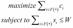
The aforementioned problem can be solved using dynamic programming, which stores the subproblem solution in a table that can be reused repeatedly while searching for an optimal solution. However, it will require more space to store the results of the subproblem. The implementation of this problem using dynamic programming is as follows:
knapsack_DP<-function(W, S, C, n){
  require(pracma)
  K<-zeros(n+1, W+1)
  for(i in 1:(n+1)){
    for(j in 1:(W+1)){
      if(i==1 | j==1){
        K[i,j]=0
      } else if(S[i-1] <= j){
        K[i, j] = max(C[i-1] + K[i-1, (j-S[i-1])],  K[i-1, j])
      } else
      {
        K[i, j] = K[i-1, j]
      }
    }
  }
  return(K[n+1, W+1])
}
The problem requires us to search for the solution in a two-dimension computation of the file and the storage required. The matrix K stores intermediate results, which can be reused to satisfy the objective under given constraints.
The All Pairs Shortest Path (APSP) problem focuses on finding the shortest path between all pairs of vertices. Let's consider a directed graph G(V, E), where for each edge ![]() , the distance d(u, v) is associated if the edges u and v are connected. For example, d(A, B) = 8 units, as shown in Figure 9.6:
, the distance d(u, v) is associated if the edges u and v are connected. For example, d(A, B) = 8 units, as shown in Figure 9.6:

Figure 9.6: DAG representation for generating Fibonacci series
The APSP algorithm will determine the shortest path to reach from one edge to the other. For example, the shortest path to reach edge B from A is A -> E -> B with a distance of 4 units. The d(u, v) in graph G is defined as follows:

One of the approaches to solve the APSP problem is by using the Floyd-Warshall algorithm, which uses dynamic programming. The approach is based on the observation that any path linking two vertices u and v may have zero or more vertices between them, defining a path. The R implementation of the Floyd-Warshall algorithm is as follows:
# Implementation of Floyd-Warshall algorithm
floydWarshall<-function(graph){
  nodes<-names(graph)
  dist<-graph
  for (n in nodes){
    for(ni in nodes){
      for(nj in nodes){
        if((dist[[ni]][n]+dist[[n]][nj])<dist[[ni]][nj]){
          dist[[ni]][nj]<-dist[[ni]][n]+dist[[n]][nj]
        }
      }
    }
  }
  return(dist)
}
The implementation begins by disallowing all intermediate vertices, thus, the initial solution is simply an initial distance matrix achieved by assigning graph to the dist list. The algorithm then proceeds by introducing an additional intermediate vertex at each step and selecting the shortest path by comparing it with the previous best estimate. The approach breaks the problem into subproblems, as the shortest distance d(u, v) between the vertices u and v, passing through vertex k, is the sum of the shortest distance d(u, k) and d(k, v). The Floyd-Warshall implementation requires a computational effort of O(n3). The APSP problem output for the graph shown in Table 9.1 can be determined using the following example script:
# Defining graph structure
graph<-list()
graph[["A"]]=c("A"=0, "B"=8, "C"=Inf, "D"=Inf, "E"=1, "F"=Inf)
graph[["B"]]=c("A"=Inf, "B"=0, "C"=7, "D"=6, "E"=Inf, "F"=Inf)
graph[["C"]]=c("A"=Inf, "B"=Inf, "C"=0, "D"=6, "E"=Inf, "F"=Inf)
graph[["D"]]=c("A"=Inf, "B"=Inf, "C"=Inf, "D"=0, "E"=Inf, "F"=4)
graph[["E"]]=c("A"=Inf, "B"=3, "C"=Inf, "D"=Inf, "E"=0, "F"=9)
graph[["F"]]=c("A"=Inf, "B"=3, "C"=Inf, "D"=4, "E"=9, "F"=0)
APSP_Dist<-floydWarshall(graph) # get shortest pair distance
The graph is stored as a list in R, which can be called using edge name. Similarly, the outcome is returned as a list object. The output from the Floyd-Warshall algorithm is shown in Table 9.1:

Table 9.1: Output from the Floyd-Warshall algorithm as the shortest distance between nodes
The Inf in the preceding table shows that there is no direct or indirect connection between the two nodes.