
In this chapter, we will introduce indexing concepts, which are essential in file structuring to organize large data on disk. Indexing also helps in attaining efficiency in data access, data search, and memory allocation. This chapter will build the foundation of indexing, and cover various type of indexing, such as linear indexing, Indexed Sequential Access Method (ISAM), and tree-based indexing. The chapter introduces linear indexing and ISAM concepts (which are an improvement over linear indexing) using R. The current chapter will also cover advanced tree-based indexing data structures. The following is the list of topics that will be covered in detail:
- 2-3 trees
- B-trees
- B+ trees
Indexing is defined as the process of associating a key with data location. The basic field of a data index includes a search key and a pointer. The search key is set of attributes that is used to look up records from a file and the pointer stores the address of the data stored in memory. The index file consists of records, also known as index entries, of the form shown in Figure. 7.1:

Figure 7.1: Example of index entries
Indexing helps in organizing a large dataset. A database has the following generic properties:
- The records are in a structured tabular format
- Records are searched using single or a combination of keys
- Aggregation queries such as sum, min, max, and average are used to summarize the dataset
Indexing in databases is used to enforce a uniqueness into records, which helps in speedy access of data. A database can have several filesystems associated with it by using indexing. This is shown in Figure 7.2 using a store database example. The store database consists of three tables: the Customer table, which stores all customer-related information, the Order table, which stores transactional level information for all orders placed by customers, and the Employee table, which stores all employee-related information:

Figure 7.2: Example of store database
All tables in the store database can be mapped together using primary, secondary, or foreign keys. The columns in the database can be classified as follows:
- Primary key: The primary key is the column which uniquely identifies each row in the table. For example,
CustomerID,OrderID, andEmployeeIDact as primary keys in the tablesCustomer,Order, andEmployeerespectively. - Secondary key: The secondary keys are one or more columns which do not have a unique sequence. For example,
FirstNameandLastNamein theEmployeetable are not able to uniquely represent each row of the table, and a second field will be required to make this column act as the primary key. Secondary keys can be used for indexing in M-dimensional feature space. - Foreign key: A foreign key is the column that points to the primary key in other tables. For example,
CustomerIDandEmployeeIDin the tableOrderact as foreign keys. This key provides an interface for a smooth interaction with other tables in the database.
In linear indexing, the keys are stored in a sorted order, and the value of the key can point to the following:
- A record stored in the filesystem
- Primary key of the dataset
- Values of the primary key
The indexes can be stored in the main memory or storage disk depending on the size of data and the keys required to map it. For example, a linear index generated based on sequence is shown in Figure 7.3:

Figure 7.3: Example of linear indexing on sequence
A linear index contains the key field, and each key field has an associated pointer which links it with the actual dataset position. The sorting of the index allows an efficient search query using binary search. Binary search locates the pointers to the disk blocks or records in the file with specific key indices. As data size increases, storing the index in the main memory would not be feasible. To deal with the issue, one solution is to store the index in the hard disk. However, this would make search an expensive process, making the current indexing approach inefficient. The current issue could be addressed by using a multi-level linear index. Multi-level indexes utilize the sorted index property and computation property of binary search to minimize computation time. The computational property of binary search requires log2bi block accesses to search for an index with bi block. Each step performed during binary search reduces the search part of the index file by a factor of 2.
Multi-level indexing utilizes this property to reduce the part of the index to be searched by a larger blocking factor, also known as fan-out (fo, where fo is greater than 2), thus improving the search to logfobi. For fo equal to 2, there is no computational improvement due to multi-level indexing. An example of second-level linear indexing is shown in Figure 7.4.
Figure 7.4 demonstrates a second-level linear indexing in which the first base level is the usual-ordered primary index with a distinct value for each key. Similarly, the second base level is a primary index for the first level. The second level is the block anchor, that is, it has a one entry for each block in the first level:
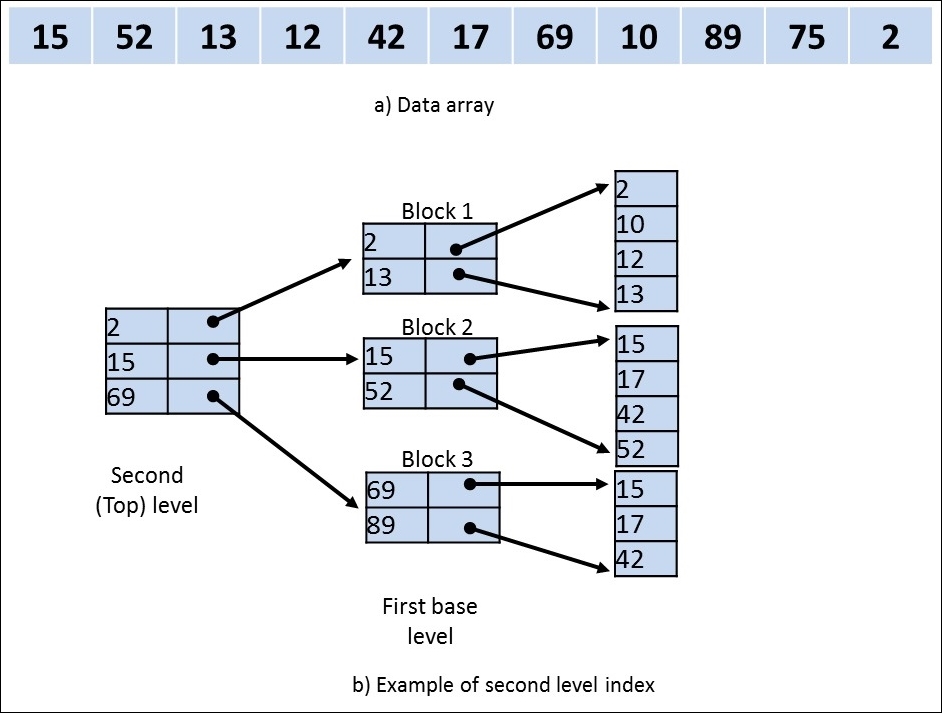
Figure 7.4: Example of a second-level linear index
The blocking factor or fan-out parameter for all levels is kept the same during indexing. Thus, if the first level has n1 entries, then the blocking factor is bf, which is also the fan-out factor fo; so, the first level needs (n1/fo) blocks, which is also the number of entries needed for the second level. Thus, with each addition of a level, the number of blocks is reduced by the fan-out factor. This approach can be repeated as many times to create a multi-level indexing, and is repeated until only one block is needed to fit all the indexes. Multi-level linear indexing can be used on any type of index, such as primary, secondary, or clustering, until the first-level index is represented with distinct keys. Linear indexing is quite efficient in structuring datasets. However, the main drawback is that any insertion or deletion operation would require a big change in the linear index, which would affect the computation effort significantly.