Chapter 3: AutoML with Amazon SageMaker Autopilot

In the previous chapter, you learned how Amazon SageMaker helps you build and prepare datasets. In a typical machine learning project, the next step would be to start experimenting with algorithms in order to find an early fit and get a sense of the predictive power you could expect from the model.

Whether you work with statistical machine learning or deep learning, three options are available when it comes to selecting an algorithm:

• Write your own, or customize an existing one. This only makes sense if you have strong skills in statistics and computer science, if you're quite sure that you can do better than well-tuned, off-the-shelf algorithms, and if you're given enough time to work on the project. Let's face it, these conditions are rarely met.
• Use a built-in algorithm implemented in one of your favorite libraries, such as Linear Regression or XGBoost. For deep learning problems, this includes pretrained models available in TensorFlow, PyTorch, and so on. This option saves you the trouble of writing machine learning code. Instead, it lets you focus on feature engineering and model optimization.
• Use AutoML, a rising technique that lets you automatically build, train, and optimize machine learning models.

In this chapter, you will learn about Amazon SageMaker Autopilot, an AutoML capability part of Amazon SageMaker. We'll see how to use it in Amazon SageMaker Studio, without writing a single line of code, and also how to use it with the Amazon SageMaker SDK:

• Discovering Amazon SageMaker Autopilot
• Using Amazon SageMaker Autopilot in SageMaker Studio
• Using Amazon SageMaker Autopilot with the SageMaker SDK
• Diving deep on Amazon SageMaker Autopilot

Technical requirements

You will need an AWS account to run examples included in this chapter. If you haven't got one already, please point your browser at https://aws.amazon.com/getting-started/ to create it. You should also familiarize yourself with the AWS Free Tier (https://aws.amazon.com/free/), which lets you use many AWS services for free within certain usage limits.

You will need to install and configure the AWS Command-Line Interface (CLI) for your account (https://aws.amazon.com/cli/).

You will need a working Python 3.x environment. Be careful not to use Python 2.7, as it is no longer maintained. Installing the Anaconda distribution (https://www.anaconda.com/) is not mandatory, but is strongly encouraged as it includes many projects that we will need (Jupyter, pandas, numpy, and more).

Code examples included in the book are available on GitHub at https://github.com/PacktPublishing/Learn-Amazon-SageMaker. You will need to install a Git client to access them (https://git-scm.com/).

Discovering Amazon SageMaker Autopilot

Added to Amazon SageMaker in late 2019, Amazon SageMaker Autopilot is an AutoML capability that takes care of all machine learning steps for you. You only need to upload a columnar dataset to an Amazon S3 bucket, and define the column you want the model to learn (the target attribute). Then, you simply launch an Autopilot job, with either a few clicks in the SageMaker Studio GUI, or a couple of lines of code with the SageMaker SDK.

The simplicity of SageMaker Autopilot doesn't come at the expense of transparency and control. You can see how your models are built, and you can keep experimenting to refine results. In that respect, SageMaker Autopilot should appeal to new and seasoned practitioners alike.

In this section, you'll learn about the different steps of a SageMaker Autopilot job, and how they contribute to delivering high-quality models:

• Analyzing data
• Feature engineering
• Model tuning

Let's start by seeing how SageMaker Autopilot analyzes data.

Analyzing data

This step is first responsible for understanding what type of machine learning problem we're trying to solve. SageMaker Autopilot currently supports linear regression, binary classification, and multi-class classification.

Note:

A frequent question is "how much data is needed to build such models?". This is a surprisingly difficult question. The answer—if there is one—depends on many factors, such as the number of features and their quality. As a basic rule of thumb, some practitioners recommend having 10-100 times more samples than features. In any case, I'd advise you to collect no fewer than hundreds of samples (for each class, if you're building a classification model). Thousands or tens of thousands are better, especially if you have more features. For statistical machine learning, there is rarely a need for millions of samples, so start with what you have, analyze the results, and iterate before going on a data collection rampage!

By analyzing the distribution of the target attribute, SageMaker Autopilot can easily figure out which one is the right one. For instance, if the target attribute has only two values (say, yes and no), it's pretty likely that you're trying to build a binary classification model.

Then, SageMaker Autopilot computes statistics on the dataset and on individual columns: the number of unique values, the mean, median, and so on. Machine learning practitioners very often do this in order to get a first feel for the data, and it's nice to see it automated. In addition, SageMaker Autopilot generates a Jupyter notebook, the data exploration notebook, to present these statistics in a user-friendly way.

Once SageMaker Autopilot has analyzed the dataset, it builds ten candidate pipelines that will be used to train candidate models. A pipeline is a combination of the following:

• A data processing job, in charge of feature engineering. As you can guess, this job runs on Amazon SageMaker Processing, which we studied in Chapter 2, Handling Data Preparation Techniques.
• A training job, running on the processed dataset. The algorithm is selected automatically by SageMaker Autopilot based on the problem type.

Next, let's see how Autopilot can be used in feature engineering.

Feature engineering

This step is responsible for preprocessing the input dataset according to the pipelines defined during data analysis.

The ten candidate pipelines are fully documented in another auto-generated notebook, the candidate generation notebook. This notebook isn't just descriptive: you can actually run its cells, and manually reproduce the steps performed by SageMaker Autopilot. This level of transparency and control is extremely important, as it lets you understand exactly how the model was built. Thus, you're able to verify that it performs the way it should, and you're able to explain it to your stakeholders. Also, you can use the notebook as a starting point for additional optimization and tweaking if you're so inclined.

Lastly, let's take a look at model tuning in Autopilot.

Model tuning

This step is responsible for training and tuning models according to the pipelines defined during data analysis. For each pipeline, SageMaker Autopilot will launch an automatic model tuning job (we'll cover this topic in detail in a later chapter). In a nutshell, each tuning job will use hyperparameter optimization to train a large number of increasingly accurate models on the processed dataset. As usual, all of this happens on managed infrastructure.

Once the model tuning is complete, you can view the model information and metrics in Amazon SageMaker Studio, build visualizations, and so on. You can do the same programmatically with the Amazon SageMaker Experiments SDK.

Finally, you can deploy your model of choice just like any other SageMaker model using either the SageMaker Studio GUI or the SageMaker SDK.

Now that we understand the different steps of an Autopilot job, let's run a job in SageMaker Studio.

Using SageMaker Autopilot in SageMaker Studio

We will build a model using only SageMaker Studio. We won't write a line of machine learning code, so get ready for zero-code AI.

In this section, you'll learn how to do the following:

• Launch a SageMaker Autopilot job in SageMaker Studio.
• Monitor the different steps of the job.
• Visualize models and compare their properties.

Launching a job

First, we need a dataset. We'll reuse the direct marketing dataset used in Chapter 2, Handling Data Preparation Techniques. This dataset describes a binary classification problem: will a customer accept a marketing offer, yes or no? It contains a little more than 41,000 labeled customer samples. Let's dive in:

1. Let's open SageMaker Studio, and create a new Python 3 notebook using the Data Science kernel, as shown in the following screenshot:
   

   Figure 3.1 – Creating a notebook

2. Now, let's download and extract the dataset as follows:

   %%sh

   apt-get -y install unzip

   wget -N https://sagemaker-sample-data-us-west-2.s3-us-west-2.amazonaws.com/autopilot/direct_marketing/bank-additional.zip

   unzip -o bank-additional.zip

3. In Chapter 2, Handling Data Preparation Techniques, we ran a feature engineering script with Amazon SageMaker Processing. We will do no such thing here: we simply upload the dataset as is to S3, into the default bucket created by SageMaker:

   import sagemaker

   prefix = 'sagemaker/DEMO-autopilot/input'sess   = sagemaker.Session()

   uri = sess.upload_data(path="./bank-additional/bank-additional-full.csv", key_prefix=prefix)

   print(uri)

   The dataset will be available in S3 at the following location:

   s3://sagemaker-us-east-2-123456789012/sagemaker/DEMO-autopilot/input/bank-additional-full.csv

4. Now, we click on the flask icon in the left-hand vertical icon bar. This opens the Experiments tab, and we click on the Create Experiment button to create a new Autopilot job.
5. The next screen is where we configure the job. As shown in the following screenshot, we first give it the name of my-first-autopilot-job:
   

   Figure 3.2 – Creating an Autopilot Experiment

   We set the location of the input dataset using the path returned in step 3. As is visible in the following screenshot, we can either browse S3 buckets or enter the S3 location directly:

   

   Figure 3.3 – Defining the input location

6. The next step is to define the name of the target attribute, as shown in the following screenshot. The column storing the yes or no label is called y:
   

   Figure 3.4 – Defining the target attribute

   As shown in the following screenshot, we set the output location where job artifacts will be copied to: s3://sagemaker-us-east-2-123456789012/sagemaker/DEMO-autopilot/output/:

   

   Figure 3.5 – Defining the output location

7. We set the type of job we want to train, as shown in the next screenshot. Here, we select Auto in order to let SageMaker Autopilot figure out the problem type. Alternatively, we could select Binary classification, and pick either the Accuracy (the default setting) or the F1 metric:
   

   Figure 3.6 – Setting the problem type

8. Finally, we decide whether we want to run a full job, or simply generate notebooks. We'll go with the former, as shown in the following screenshot. The latter would be a good option if we wanted to train and tweak the parameters manually:
   

   Figure 3.7 – Running a complete experiment

9. Optionally, in the Advanced Settings section, we would change the IAM role, set an encryption key for job artifacts, and define the VPC where we'd like to launch job instances. Let's keep default values here.
10. The job setup is complete: all it took was this one screen. Then, we click on Create Experiment, and off it goes!

Monitoring a job

Once the job is launched, it goes through the three steps that we already discussed, which should take around 5 hours to complete. The new experiment is listed in the Experiments tab, and we can right-click Describe AutoML Job to describe its current status. This opens the following screen, where we can see the progress of the job:

1. As expected, the job starts by analyzing data, as highlighted in the following screenshot:
   

   Figure 3.8 – Viewing job progress

2. About 10 minutes later, the data analysis is complete, and the job moves on to feature engineering. As shown in the next screenshot, we can also see new two buttons in the top-right corner, pointing at the candidate generation and data exploration notebooks; don't worry, we'll take a deeper look at both later in the chapter:
   

   Figure 3.9 – Viewing job progress

3. Once feature engineering is complete, the job then moves on the model tuning. As visible in the following picture, we see the first models being trained in the Trials tab. A trial is the name Amazon SageMaker Experiments uses for a collection of related jobs, such as processing jobs, batch transform jobs, training jobs, and so on:
   

   Figure 3.10 – Viewing tuning jobs

4. At first, we see ten tuning jobs, corresponding to the ten candidate pipelines. Once a job is complete, we can see its Objective, that is to say, the metric that the job tried to optimize (in this case, it's the validation accuracy). We can sort jobs based on this metric, and the best tuning job so far is highlighted with a star. Your screen should look similar to the following screenshot:
   

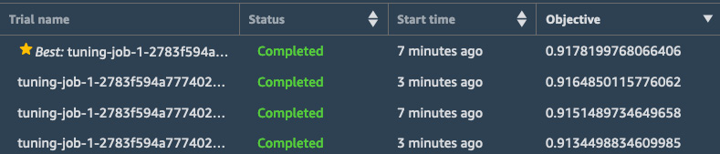
   Figure 3.11 – Viewing results

5. If we select a job and right-click Open in trial details, we can see plenty of additional information, such as the other jobs that belong to the same trial. In the following screenshot, we also see the actual algorithm that was used for training (XGBoost) along with its hyperparameter values:
   

   Figure 3.12 – Examining a job

6. After several hours, the SageMaker Autopilot job is complete. 500 jobs have been trained. This is a default value that can be changed in the SageMaker API.

At this point, we could simply deploy the top job, but instead, let's compare the top ten ones using the visualization tools built into SageMaker Studio.

Comparing jobs

A single SageMaker Autopilot job trains hundreds of jobs. Over time, you may end up with tens of thousands of jobs, and you may wish to compare their properties. Let's see how:

1. Going to the Experiments tab on the left, we locate our job and right-click Open in trial component list, as visible in the following screenshot:
   

   Figure 3.13 – Comparing jobs

2. This opens the Trial Component List, as shown in the following screenshot.

   We open the Table Properties panel on the right by clicking on the icon representing a cog. In the Metrics section, we tick the ObjectiveMetric box. In the Type filter section, we only tick Training job. In the main panel, we sort jobs by descending objective metric by clicking on the arrow. We hold Shift and click the top ten jobs to select them. Then, we click on the Add chart button:

   

   Figure 3.14 – Comparing jobs

3. This opens the Trial Component Chart tab, as visible in the screenshot that follows. Click inside the chart box at the bottom to open the Chart properties panel on the right:
   

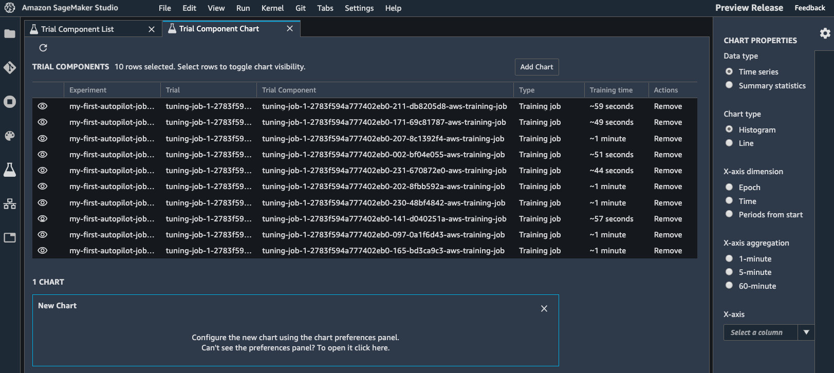
   Figure 3.15 – Comparing jobs

   As our training jobs are very short (about a minute), there won't be enough data for Time series charts, so let's select Summary statistics instead. We're going to build a scatter plot, putting the maximum training accuracy and validation accuracy in perspective, as shown in the following screenshot. We also color data points with our trial names:

   

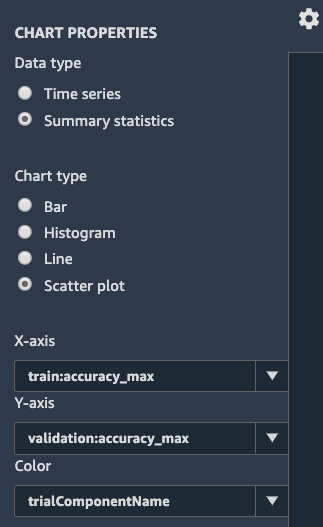
   Figure 3.16 – Creating a chart

4. Zooming in on the following chart, we can quickly visualize our jobs and their respective metrics. We could build additional charts showing the impact of certain hyperparameters on accuracy. This would help us shortlist a few models for further testing. Maybe we would end up considering several of them for ensemble prediction:

Figure 3.17 – Plotting accuracies

The next step is to deploy a model and start testing it.

Deploying and invoking a model

The SageMaker Studio GUI makes it extremely easy to deploy a model. Let's see how:

1. Going back to the Experiments tab, we right-click the name of our experiment and select Describe AutoML Job. This opens the list of training jobs. Making sure that they're sorted by descending objective, we select the best one (it's highlighted with a star), as shown in the screenshot that follows, and then we click on the Deploy model button:
   

   Figure 3.18 – Deploying a model

2. On the screen shown in the following screenshot, we just give the endpoint name and leave all other settings as is. The model will be deployed on a real-time HTTPS endpoint backed by an ml.m5.xlarge instance:
   

   Figure 3.19 – Deploying a model

3. Heading to the Endpoints section in the left-hand vertical panel, we can see the endpoint being created. As shown in the following screenshot, it will initially be in the Creating state. After a few minutes, it will be In service:
   

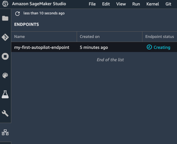
   Figure 3.20 – Creating an endpoint

4. Moving to a Jupyter notebook (we can reuse the one we wrote to download the dataset), we define the name of the endpoint, and a sample to predict. Here, I'm using the first line of the dataset:

   ep_name = 'my-first-autopilot-endpoint'

   sample = '56,housemaid,married,basic.4y,no,no,no,telephone,may,mon,261,1,999,0,nonexistent,1.1,93.994,-36.4,4.857,5191.0'

5. We create a boto3 client for the SageMaker runtime. This runtime contains a single API, invoke_endpoint (https://boto3.amazonaws.com/v1/documentation/api/latest/reference/services/sagemaker-runtime.html). This makes it efficient to embed in client applications that just need to invoke models:

   import boto3

   sm_rt = boto3.Session().client('runtime.sagemaker')

6. We send the sample to the endpoint, also passing the input and output content types:

   response = sm_rt.invoke_endpoint(EndpointName=ep_name,                              ContentType='text/csv',                              Accept='text/csv',                              Body=sample)

7. We decode the prediction and print it – this customer is not likely to accept the offer:

   response = response['Body'].read().decode("utf-8")print(response)

   This sample is predicted as a no:

   no

8. When we're done testing the endpoint, we should delete it to avoid unnecessary charges. We can do this with the delete_endpoint API in boto3 (https://boto3.amazonaws.com/v1/documentation/api/latest/reference/services/sagemaker.html#SageMaker.Client.delete_endpoint):

   sm = boto3.Session().client('sagemaker')sm.delete_endpoint(EndpointName=ep_name)

Congratulations, you've successfully built, trained, and deployed your first machine learning model on Amazon SageMaker. That was pretty simple, wasn't it? The only code we wrote was to download the dataset and to predict with our model.

Using the SageMaker Studio GUI is a great way to quickly experiment with a new dataset, and also to let less technical users build models on their own. Now, let's see how we can use SageMaker Autopilot programmatically with the SageMaker SDK.

Using the SageMaker Autopilot SDK

The Amazon SageMaker SDK includes a simple API for SageMaker Autopilot. You can find its documentation at https://sagemaker.readthedocs.io/en/stable/automl.html.

In this section, you'll learn how to use this API to train a model on the same dataset as in the previous section.

Launching a job

The SageMaker SDK makes it extremely easy to launch an Autopilot job – just upload your data in S3, and call a single API! Let's see how:

1. First, we import the SageMaker SDK:

   import sagemaker

   sess = sagemaker.Session()

2. Then, we download the dataset:

   %%sh

   wget -N https://sagemaker-sample-data-us-west-2.s3-us-west-2.amazonaws.com/autopilot/direct_marketing/bank-additional.zip unzip -o bank-additional.zip

3. Next, we upload the dataset to S3:

   bucket = sess.default_bucket()                     prefix = 'sagemaker/DEMO-automl-dm'

   s3_input_data = upload_data(path="./bank-additional/bank-additional-full.csv", key_prefix=prefix+'input')

4. We then configure the AutoML job, which only takes one line of code. We define the target attribute (remember, that column is named y), and where to store training artifacts. Optionally, we can also set a maximum run time for the job, a maximum run time per job, or reduce the number of candidate models that will be tuned. Please note that restricting the job's duration too much is likely to impact its accuracy. For development purposes, this isn't a problem, so let's cap our job at one hour, or 250 tuning jobs (whichever limit it hits first):

   from sagemaker.automl.automl import AutoML

   auto_ml_job = AutoML(    role = sagemaker.get_execution_role(),    sagemaker_session = sess,    target_attribute_name = 'y',    output_path =     's3://{}/{}/output'.format(bucket,prefix),    max_runtime_per_training_job_in_seconds = 600,    max_candidates = 250,    total_job_runtime_in_seconds = 3600 )

5. Next, we launch the Autopilot job, passing it the location of the training set. We turn logs off (who wants to read hundreds of tuning logs?), and we set the call to non-blocking, as we'd like to query the job status in the next cells:

   auto_ml_job.fit(inputs=s3_input_data, logs=False, wait=False)

The job starts right away. Now let's see how we can monitor its status.

Monitoring a job

While the job is running, we can use the describe_auto_ml_job() API to monitor its progress:

1. For example, the following code will check the job's status every 30 seconds until the data analysis step completes:

   from time import sleep

   job = auto_ml_job.describe_auto_ml_job()job_status = job['AutoMLJobStatus']job_sec_status = job['AutoMLJobSecondaryStatus']

   if job_status not in ('Stopped', 'Failed'):    while job_status in ('InProgress') and job_sec_status     in ('AnalyzingData'):

           sleep(30)        job = auto_ml_job.describe_auto_ml_job()        job_status = job['AutoMLJobStatus']        job_sec_status = job['AutoMLJobSecondaryStatus']        print (job_status, job_sec_status)

2. Once the data analysis is complete, the two auto-generated notebooks are available. We can find their location using the same API:

   job = auto_ml_job.describe_auto_ml_job()

   job_candidate_notebook = job['AutoMLJobArtifacts']['CandidateDefinitionNotebookLocation']

   job_data_notebook = job['AutoMLJobArtifacts']['DataExplorationNotebookLocation']

   print(job_candidate_notebook)print(job_data_notebook)

   This prints out the S3 paths for the two notebooks:

   s3://sagemaker-us-east-2-123456789012/sagemaker/DEMO-automl-dm/output/automl-2020-04-24-14-21-16-938/sagemaker-automl-candidates/pr-1-a99cb56acb5945d695c0e74afe8ffe3ddaebafa94f394655ac973432d1/notebooks/SageMakerAutopilotCandidateDefinitionNotebook.ipynb

   s3://sagemaker-us-east-2-123456789012/sagemaker/DEMO-automl-dm/output/automl-2020-04-24-14-21-16-938/sagemaker-automl-candidates/pr-1-a99cb56acb5945d695c0e74afe8ffe3ddaebafa94f394655ac973432d1/notebooks/SageMakerAutopilotDataExplorationNotebook.ipynb

3. Using the AWS CLI, we can copy the two notebooks locally. We'll take a look at them later in this chapter:

   %%sh -s $job_candidate_notebook $job_data_notebook

   aws s3 cp $1 .aws s3 cp $2 .

4. While the feature engineering runs, we can wait for completion using the same code snippet as the preceding, looping while job_sec_status is equal to FeatureEngineering.
5. Once the feature engineering is complete, the model tuning starts. While it's running, we can use the Amazon SageMaker Experiments SDK to keep track of jobs. We'll cover SageMaker Experiments in detail in a later chapter, but here, the code is simple enough to give you a sneak peek! All it takes is to pass the experiment name to the ExperimentAnalytics object. Then, we can retrieve information on all tuning jobs so far in a pandas DataFrame. From then on, it's business as usual, and we can easily display the number of jobs that have already run, and the top 5 jobs so far:

   import pandas as pd

   from sagemaker.analytics import ExperimentAnalytics

   exp = ExperimentAnalytics(    sagemaker_session=sess,    experiment_name=job['AutoMLJobName'] +                     '-aws-auto-ml-job')

   df = exp.dataframe()print("Number of jobs: ", len(df))

   df = pd.concat([df['ObjectiveMetric - Max'], df.drop(['ObjectiveMetric - Max'], axis=1)], axis=1)

   df.sort_values('ObjectiveMetric - Max', ascending=0)[:5]

   This pandas code outputs the following table:

   

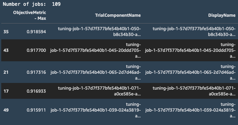
   Figure 3.21 – Viewing jobs

6. Once the model tuning is complete, we can very easily find the best candidate:

   job_best_candidate = auto_ml_job.best_candidate()

   print(job_best_candidate['CandidateName'])print(job_best_candidate['FinalAutoMLJobObjectiveMetric'])

   This prints out the name of the best tuning job, along with its validation accuracy:

   tuning-job-1-57d7f377bfe54b40b1-030-c4f27053

   {'MetricName': 'validation:accuracy', 'Value': 0.9197599935531616}

Then, we can deploy and test the model using the SageMaker SDK. We've covered a lot of ground already, so let's save that for future chapters, where we'll revisit this example.

Cleaning up

SageMaker Autopilot creates many underlying artifacts such as dataset splits, pre-processing scripts, pre-processed datasets, models, and so on. If you'd like to clean up completely, the following code snippet will do that. Of course, you could also use the AWS CLI:

import boto3

job_outputs_prefix = '{}/output/{}'.format(prefix, job['AutoMLJobName'])

s3_bucket = boto3.resource('s3').Bucket(bucket)s3_bucket.objects.filter(Prefix=job_outputs_prefix).delete()

Now that we know how to train models using both the SageMaker Studio GUI and the SageMaker SDK, let's take a look under the hood. Engineers like to understand how things really work, right?

Diving deep on SageMaker Autopilot

In this section, we're going to learn in detail how SageMaker Autopilot processes data and trains models. If this feels too advanced for now, you're welcome to skip this material. You can always revisit it later once you've gained more experience with the service.

First, let's look at the artifacts that SageMaker Autopilot produces.

The job artifacts

Listing our S3 bucket confirms the existence of many different artifacts:

$ aws s3 ls s3://sagemaker-us-east-2-123456789012/sagemaker/DEMO-autopilot/output/my-first-autopilot-job/

We can see many new prefixes. Let's figure out what's what:

PRE data-processor-models/PRE preprocessed-data/PRE sagemaker-automl-candidates/PRE transformed-data/PRE tuning/

The preprocessed-data/tuning_data prefix contains the training and validation splits generated from the input dataset. Each split is further broken into small CSV chunks:

• The sagemaker-automl-candidates prefix contains ten data preprocessing scripts (dpp[0-9].py), one for each pipeline. It also contains the code to train them (trainer.py) on the input dataset, and the code to process the input dataset with each one of the ten resulting models (sagemaker_serve.py).
• The data-processor-models prefix contains the ten data processing models trained by the dpp scripts.
• The transformed-data prefix contains the ten processed versions of the training and validation splits.
• The sagemaker-automl-candidates prefix contains the two auto-generated notebooks.
• Finally, the tuning prefix contains the actual models trained during the Model Tuning step.

The following diagram summarizes the relationship between these artifacts:

Figure 3.22 – Summing up the Autopilot process

In the next sections, we'll take a look at the two auto-generated notebooks, which are one of the most important features in SageMaker Autopilot.

The Data Exploration notebook

This notebook is available in Amazon S3 once the data analysis step is complete.

The first section, seen in the following screenshot, simply displays a sample of the dataset:

Figure 3.23 – Viewing dataset statistics

Shown in the following screenshot, the second section focuses on column analysis: percentages of missing values, counts of unique values, and descriptive statistics. For instance, it appears that the pdays field has both a maximum value and a median of 999, which looks suspicious. As explained in the previous chapter, 999 is indeed a placeholder value meaning that a customer has never been contacted before:

Figure 3.24 – Viewing dataset statistics

As you can see, this notebook saves us the trouble of computing these statistics ourselves, and we can use them to quickly check that the dataset is what we expect.

Now, let's look at the second notebook. As you will see, it's extremely insightful!

The Candidate Generation notebook

This notebook contains the definition of the ten candidate pipelines, and how they're trained. This is a runnable notebook, and advanced practitioners can use it to replay the AutoML process, and keep refining their experiment. Please note that this is totally optional! It's perfectly OK to deploy the top model directly and start testing it.

Having said that, let's run one of the pipelines manually:

1. We open the notebook and save a read-write copy by clicking on the Import notebook link in the top-right corner.
2. Then, we run the cells in the SageMaker Setup section to import all required artifacts and parameters.
3. Moving to the Candidate Pipelines section, we create a runner object that will launch jobs for selected candidate pipelines:

   from sagemaker_automl import AutoMLInteractiveRunner, AutoMLLocalCandidate

   automl_interactive_runner = AutoMLInteractiveRunner(AUTOML_LOCAL_RUN_CONFIG)

4. Then, we add the first pipeline (dpp0). The notebook tells us: "This data transformation strategy first transforms 'numeric' features using RobustImputer (converts missing values to nan), 'categorical' features using ThresholdOneHotEncoder. It merges all the generated features and applies RobustStandardScaler. The transformed data will be used to tune a xgboost model." We just need to run the following cell to add it:

   automl_interactive_runner.select_candidate(    {"data_transformer": {        "name": "dpp0",        …    })

   If you're curious about the implementation of RobustImputer or ThresholdOneHotEncoder, hyperlinks take you to the appropriate source file in the sagemaker_sklearn_extension module (https://github.com/aws/sagemaker-scikit-learn-extension/).

   This way, you can understand exactly how data has been processed. As these objects are based on scikit-learn objects, they should quickly look very familiar. For instance, we can see that RobustImputer is built on top of sklearn.impute.SimpleImputer, with added functionality. Likewise, ThresholdOneHotEncoder is an extension of sklearn.preprocessing.OneHotEncoder.

5. Taking a quick look at other pipelines, we see different processing strategies and algorithms. You should see the Linear Learner algorithm used in some pipelines: it's one of the built-in algorithms in SageMaker, and we'll cover it in the next chapter.
6. Scrolling down, we get to the Selected Candidates section, where we can indeed confirm that we have only selected the first pipeline:

   automl_interactive_runner.display_candidates()

   This is visible in the result here:

   

   This also tells us that data will be processed by the dpp0.py script, and that the model will be trained using the XGBoost algorithm.

7. Clicking on the dpp0 hyperlink opens the script. As expected, we see that it builds a scikit-learn transformer pipeline (not to be confused with the SageMaker pipeline composed of preprocessing and training jobs). Missing values are imputed in the numerical features, and the categorical features are one-hot encoded. Then, all features are scaled and the labels are encoded:

   numeric_processors = Pipeline(  steps=[('robustimputer',         RobustImputer(strategy='constant',                       fill_values=nan))])

   categorical_processors = Pipeline(  steps=[('thresholdonehotencoder',          ThresholdOneHotEncoder(threshold=301))])

   column_transformer = ColumnTransformer(  transformers=[    ('numeric_processing', numeric_processors, numeric),    ('categorical_processing', categorical_processors,        categorical)])

   return Pipeline(steps=[  ('column_transformer', column_transformer),     ('robuststandardscaler', RobustStandardScaler())])

8. Back in the notebook, we launch this script in the Run Data Transformation Steps section:

   automl_interactive_runner.fit_data_transformers(parallel_jobs=7)

9. This creates two sequential SageMaker jobs, and their artifacts are stored in a new prefix created for the notebook run:

   $ aws s3 ls s3://sagemaker-us-east-2-123456789012/sagemaker/DEMO-autopilot/output/my-first-autopilot-job/my-first-a-notebook-run-24-13-17-22/

   The first job trains the dpp0 transformers on the input dataset.

   The second job processes the input dataset with the resulting model. For the record, this job uses the SageMaker Batch Transform feature, which will be covered in a later chapter.

   Going back to SageMaker Studio, let's find out more about these two jobs. Starting from the Experiments tab on the left (the flask icon, remember?), we select Unassigned trial components, and we see our two jobs there: my-first-a-notebook-run-24-13-17-22-dpp0-train-24-13-38-38-aws-training-job and my-first-a-notebook-run-24-13-17-22-dpp0-transform-24-13-38-38-aws-transform-job.

10. Double-clicking a job name opens the Describe Trial Component window, as shown in the following screenshot. It tells us everything there is to know about the job: the parameters, location of artifacts, and more:

Figure 3.25 – Describing a trial

Once data processing is complete, the notebook proceeds with automatic model tuning and model deployment. We haven't yet discussed these topics, so let's stop there for now. I encourage you to go through the rest of the notebook once you're comfortable with them.

Summary

As you can see, Amazon SageMaker Autopilot makes it easy to build, train, and optimize machine learning models for beginners and advanced users alike.

In this chapter, you learned about the different steps of an Autopilot job, and what they mean from a machine learning perspective. You also learned how to use both the SageMaker Studio GUI and the SageMaker SDK to build a classification model with minimal coding. Then, we dived deep on the auto-generated notebooks, which give you full control and transparency over the modeling processing. In particular, you learned how to run the Candidate Generation notebook manually, in order to replay all steps involved.

In the next chapter, you will learn how to use the built-in algorithms in Amazon SageMaker to train models for a variety of machine learning problems.