Chapter 5: Training Computer Vision Models

In the previous chapter, you learned how to use SageMaker's built-in algorithms for traditional machine learning problems including classification, regression, and anomaly detection. We saw that these algorithms work well on tabular data, such as CSV files. However, they are not well suited for image datasets, and they generally perform very poorly on computer vision (CV) tasks.

For a few years now, CV has taken the world by storm, and not a month goes by without a new breakthrough in extracting patterns from images and videos. In this chapter,you will learn about three built-in algorithms designed specifically for CV tasks.We'll discuss the types of problems that you can solve with them. We'll also spend a lot of time explaining how to prepare image datasets, as this crucial topic is often inexplicably overlooked. Of course, we'll train and deploy models too.

This chapter covers the following topics:

• Discovering the CV built-in algorithms in Amazon SageMaker
• Preparing image datasets
• Using the CV built-in algorithms: image classification, object detection, and semantic segmentation.

Technical requirements

You will need an AWS account to run the examples included in this chapter. If you haven't got one already, please point your browser to https://aws.amazon.com/getting-started/ to create it. You should also familiarize yourself with the AWS Free Tier (https://aws.amazon.com/free/), which lets you use many AWS services for free within certain usage limits.

You will need to install and configure the AWS Command-Line Interface (CLI) for your account (https://aws.amazon.com/cli/).

You will need a working Python 3.x environment. Be careful not to use Python 2.7, as it is no longer maintained. Installing the Anaconda distribution (https://www.anaconda.com/) is not mandatory, but strongly encouraged, as it includes many projects that we will need (Jupyter, pandas, numpy, and more).

The code examples included in the book are available on GitHub at https://github.com/PacktPublishing/Learn-Amazon-SageMaker. You will need to install a Git client to access them (https://git-scm.com/).

Discovering the CV built-in algorithms in Amazon SageMaker

SageMaker includes three CV algorithms, based on proven deep learning networks. In this section, you'll learn about these algorithms, what kind of problems they can help you solve, and what their training scenarios are:

• Image classification assigns one or more labels to an image.
• Object detection detects and classifies objects in an image.
• Semantic segmentation assigns every pixel of an image to a specific class.

Discovering the image classification algorithm

Starting from an input image, the image classification algorithm predicts a probability for each class present in the training dataset. This algorithm is based on the ResNet convolutional neural network (https://arxiv.org/abs/1512.03385). Published in 2015, ResNet won the ILSVRC classification task that same year (http://www.image-net.org/challenges/LSVRC/). Since then, it has become a popular and versatile choice for image classification.

Many hyperparameters can be set, including the depth of the network, which can range from 18 to 200 layers. In general, the more layers the network has, the better it will learn, at the expense of increased training times.

Please note that the image classification algorithm supports both single-label and multi-label classification. We will focus on single-label classification in this chapter. Working with several labels is very similar, and you'll find a complete example at https://github.com/awslabs/amazon-sagemaker-examples/blob/master/introduction_to_amazon_algorithms/imageclassification_mscoco_multi_label/.

Discovering the object detection algorithm

Starting from an input image, the object detection algorithm predicts both the class and the location of each object in the image. Of course, the algorithm can only detect object classes present in the training dataset. The location of each object is defined by a set of four coordinates, called a bounding box.

This algorithm is based on the Single Shot MultiBox Detector (SSD) architecture (https://arxiv.org/abs/1512.02325). For classification, you can pick from two base networks: VGG-16 (https://arxiv.org/abs/1409.1556) or ResNet-50.

The following output shows an example of object detection (source: https://www.dressagechien.net/wp-content/uploads/2017/11/chien-et-velo.jpg):

Figure 5.1 – Test image

Discovering the semantic segmentation algorithm

Starting from an input image, the semantic segmentation algorithm predicts the class of every pixel of the image. This is a much harder problem than image classification (which only considers the full image) or object detection (which only focuses on specific parts of the image). Using the probabilities contained in a prediction, it's possible to build segmentation masks that cover specific objects in the picture.

Three neural networks may be used for segmentation:

• Fully Convolutional Networks (FCNs): https://arxiv.org/abs/1411.4038
• Pyramid Scene Parsing (PSP): https://arxiv.org/abs/1612.01105
• DeepLab v3: https://arxiv.org/abs/1706.05587

The encoder network is ResNet, with either 50 or 101 layers.

The following output shows the result of segmenting the previous image. We see the segmentation masks, and each class is assigned a unique color; the background is black, and so on:

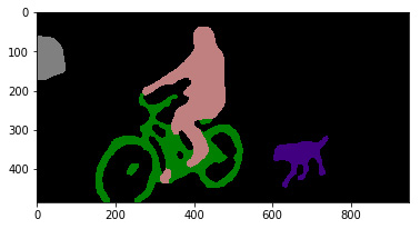
Figure 5.2 – Segmented test image

Now let's see how we can train these algorithms on our own data.

Training with CV algorithms

All three algorithms are based on supervised learning, so our starting point will be a labeled dataset. Of course, the nature of these labels will be different for each algorithm:

• Class labels for image classification
• Bounding boxes and class labels for object detection
• Segmentation masks and class labels for semantic segmentation

Annotating image datasets is a lot of work. If you need to build your own dataset, Amazon SageMaker Ground Truth can definitely help, and we studied it in Chapter 2, Handling Data Preparation Tasks. Later in this chapter, we'll show you how to use image datasets labeled with Ground Truth.

When it comes to packaging datasets, the use of RecordIO files is strongly recommended (https://mxnet.apache.org/api/faq/recordio). Packaging images in a small number of record-structured files makes it much easier to move datasets around and to split them for distributed training. Having said that, you can also train on individual image files if you prefer.

Once your dataset is ready in S3, you need to decide whether you'd like to train from scratch, or whether you'd like to start from a pretrained network.

Training from scratch is fine if you have plenty of data, and if you're convinced that there's value in building a specific model with it. However, this will take a lot of time, possibly hundreds of epochs, and hyperparameter selection will be absolutely critical in getting good results.

Using a pretrained network is generally the better option, even if you have lots of data. Thanks to transfer learning, you can start from a model trained on a huge collection of images (think millions), and fine-tune it on your data and classes. Training will be much shorter, and you will get models with higher accuracy rates quicker.

Given the complexity of the models and the size of datasets, training with CPU instances is simply not an option. We'll use GPU instances for all examples.

Last but not least, all three algorithms are based on Apache MXNet. This lets you export their models outside of SageMaker, and deploy them anywhere you like.

In the next sections, we're going to zoom in on image datasets, and how to prepare them for training.

Preparing image datasets

Input formats are more complex for image datasets than for tabular datasets, and we need to get them exactly right. The CV algorithms in SageMaker support three input formats:

• Image files
• RecordIO files
• Augmented manifests built by SageMaker Ground Truth

In this section, you'll learn how to prepare datasets in these different formats. To the best of my knowledge, this topic has rarely been addressed in such detail. Get ready to learn a lot!

Working with image files

This is the simplest format, and it's supported by all three algorithms. Let's see how to use it with the image classification algorithm.

Converting an image classification dataset to image format

A dataset in image format has to be stored in S3. Images don't need to be sorted in any way, and you simply could store all of them in the same bucket.

Images are described in a list file, a text file containing a line per image. For image classification, three columns are present: the unique identifier of the image, its class label, and its path. Here is an example:

1023  5  prefix/image2753.jpg 38    6  another_prefix/image72.jpg 983   2  yet_another_prefix/image863.jpg

The first line tells us that image2753.jpg belongs to class 5, and has been assigned ID 1023.

You need a list file for each channel, so you would need one for the training dataset, one for the validation dataset, and so on. You can either write bespoke code to generate them, or you can use a simple program that is part of Apache MXNet. This program is called im2rec, and it's available in Python and C++. We'll use the Python version.

Let's use the "Dogs vs. Cats" dataset available on Kaggle (https://www.kaggle.com/c/dogs-vs-cats). This dataset is 812 MB. Unsurprisingly, it contains two classes: dogs and cats. It's already split for training and testing (25,000 and 12,500 images, respectively). Here's how we can use it:

1. We create a Kaggle account, accept the rules of the "Dogs vs. Cats" competition, and install the kaggle CLI (https://github.com/Kaggle/kaggle-api).
2. In a Terminal, we download and extract the training dataset (you can ignore the test set, which is only needed for the competition). I recommend doing this on a Notebook instance or an EC2 instance instead of your local machine, as we'll later sync the processed dataset to S3:

   $ kaggle competitions download -c dogs-vs-cats $ unzip dogs-vs-cats.zip $ unzip train.zip

3. Dog and cat images are mixed up in the same folder. We create a subfolder for each class, and move the appropriate images there:

   $ cd train $ mkdir dog cat $ find . -name 'dog.*' -exec mv {} dog ;$ find . -name 'cat.*' -exec mv {} cat ;

4. We'll need validation images, so let's move 1,250 random dog images and 1,250 random cat images to specific directories. I'm using bash scripting here, but feel free to use any tool you like:

   $ mkdir -p val/dog val/cat $ ls dog | sort -R | tail -1250 | while read file;do mv dog/$file val/dog; done $  ls cat | sort -R | tail -1250 | while read file;do mv cat/$file val/cat; done

5. We move the remaining 22,500 images to the training folder:

   $ mkdir train $ mv dog cat train

6. Our dataset now looks like this:

   $ du -h 33M     ./val/dog 28M     ./val/cat 60M     ./val 289M    ./train/dog 248M    ./train/cat 537M    ./train 597M    .

7. We download the im2rec tool from GitHub (https://github.com/apache/incubator-mxnet/blob/master/tools/im2rec.py). It requires two dependencies, Apache MXNet and OpenCV, which we install as follows:

   $ wget https://raw.githubusercontent.com/apache/incubator-mxnet/master/tools/im2rec.py
$ pip install mxnet opencv-python

8. We run im2rec to build two list files, one for training data and one for validation data:

   $ python3 im2rec.py --list --recursive dogscats-train train $ python3 im2rec.py --list --recursive dogscats-val val

   This creates the dogscats-train.lst and dogscats-val.lst files. Their three columns are a unique image identifier, the class label (0 for cats, 1 for dogs), and the image path, as follows:

   3197 0.000000 cat/cat.1625.jpg 15084 1.000000 dog/dog.12322.jpg 1479 0.000000 cat/cat.11328.jpg 5262 0.000000 cat/cat.3484.jpg 20714 1.000000 dog/dog.6140.jpg

9. We move the list files to specific directories. This is required because they will be passed to the estimator as two new channels, train_lst and validation_lst:

   $ mkdir train_lst val_lst $ mv dogscats-train.lst train_lst $ mv dogscats-val.lst val_lst

10. The dataset now looks like this:

    $ du -h 33M     ./val/dog 28M     ./val/cat 60M     ./val 700K    ./train_lst 80K     ./val_lst 289M    ./train/dog 248M    ./train/cat 537M    ./train 597M    .

11. Finally, we sync this folder to the SageMaker default bucket for future use. Please make sure to only sync the four folders, and nothing else:

    $ aws s3 sync .   s3://sagemaker-eu-west-1-123456789012/dogscats-images/input/

Now, let's move on to using the image format with the object detection algorithms.

Converting detection datasets to image format

The general principle is identical. We need to build a file tree representing the four channels: train, validation, train_annotation, and validation_annotation.

The main difference lies in how labeling information is stored. Instead of list files, we need to build JSON files.

Here's an example of a fictitious picture in an object detection dataset. For each object in the picture, we define the coordinates of the top-left corner of its bounding box, its height, and its width. We also define the class identifier, which points to a category array that also stores class names:

{   "file": " my-prefix/my-picture.jpg",

   "image_size": [{"width": 512,"height": 512,"depth": 3}],

   "annotations": [      {       "class_id": 1,        "left": 67, "top": 121, "width": 61, "height": 128       },      {       "class_id": 5,        "left": 324, "top": 134, "width": 112, "height": 267       }   ],

   "categories": [      { "class_id": 1, "name": "pizza" },      { "class_id": 5, "name": "beer" }   ]}

We would need to do this for every picture in the dataset, building a JSON file for the training set and one for the validation set.

Finally, let's see how to use the image format with the semantic segmentation algorithm.

Converting segmentation datasets to image format

Image format is the only format supported by the image segmentation algorithm.

This time, we need to build a file tree representing the four channels: train, validation, train_annotation, and validation_annotation. The first two channels contain the source images, and the last two contain the segmentation mask images.

File naming is critical in matching an image to its mask: the source image and the mask image must have the same name in their respective channels. Here's an example:

├── train │   ├── image001.png │   ├── image007.png │   └── image042.png ├── train_annotation │   ├── image001.png │   ├── image007.png │   └── image042.png ├── validation │   ├── image059.png │   ├── image062.png │   └── image078.png └── validation_annotation │   ├── image059.png │   ├── image062.png │   └── image078.png

You can see sample pictures in the following figure. The source image on the left would go to the train folder and the mask picture on the right would go to the train_annotation folder. They should have the same name, so that the algorithm could match them.

Figure 5.3 – Sample image from the Pascal VOC dataset

One clever feature of this format is how it matches class identifiers to mask colors. Mask images are PNG files with a 256-color palette. Each class in the dataset is assigned a specific entry in the color palette. These colors are the ones you see in masks for objects belonging to that class.

If your labeling tool or your existing dataset don't support this PNG feature, you can add your own color mapping file. Please refer to the AWS documentation for details: https://docs.aws.amazon.com/sagemaker/latest/dg/semantic-segmentation.html

Now, let's prepare the Pascal VOC dataset. This dataset is frequently used to benchmark object detection and semantic segmentation models (http://host.robots.ox.ac.uk/pascal/VOC/):

1. We first download and extract the 2012 version of the dataset. Again, I recommend using an AWS-hosted instance to speed up network transfers:

   $ wget http://host.robots.ox.ac.uk/pascal/VOC/voc2012/VOCtrainval_11-May-2012.tar $ tar xvf VOCtrainval_11-May-2012.tar

2. We create a work directory where we'll build the four channels:

   $ mkdir s3_data $ cd s3_data $ mkdir train validation train_annotation validation_annotation

3. Using the list of training files defined in the dataset, we copy the corresponding images to the train folder. I'm using bash scripting here; feel free to use your tool of choice:

   $ for file in `cat ../VOCdevkit/VOC2012/ImageSets/Segmentation/train.txt | xargs`; do cp ../VOCdevkit/VOC2012/JPEGImages/$file".jpg" train; done

4. We then do the same for the validation images, training masks, and validation masks:

   $ for file in `cat ../VOCdevkit/VOC2012/ImageSets/Segmentation/val.txt | xargs`; do cp ../VOCdevkit/VOC2012/JPEGImages/$file".jpg" validation; done

   $ for file in `cat ../VOCdevkit/VOC2012/ImageSets/Segmentation/train.txt | xargs`; do cp ../VOCdevkit/VOC2012/SegmentationClass/$file".png" train_annotation; done

   $ for file in `cat ../VOCdevkit/VOC2012/ImageSets/Segmentation/val.txt | xargs`; do cp ../VOCdevkit/VOC2012/SegmentationClass/$file".png" validation_annotation; done

5. We check that we have the same number of images in the two training channels, and in the two validation channels:

   $ for dir in train train_annotation validation validation_annotation; do find $dir -type f | wc -l; done

   We see 1,464 training files and masks, and 1,449 validation files and masks.We're all set:

   1464 1464 1449 1449

6. The last step is to sync the file tree to S3 for later use. Again, please make sure to sync only the four folders:

   $ aws s3 sync . s3://sagemaker-eu-west-1-123456789012/pascalvoc-segmentation/input/

We know how to prepare classification, detection, and segmentation datasets in image format. This is a critical step, and you have to get things exactly right.

Still, I'm sure that you found the steps in this section a little painful. So did I! Now imagine doing the same with millions of images. That doesn't sound very exciting, does it?

We need an easier way to prepare image datasets. Let's see how we can simplify dataset preparation with RecordIO files.

Working with RecordIO files

RecordIO files are easier to move around. It's much more efficient for an algorithm to read a large sequential file than to read lots of tiny files stored at random disk locations.

Converting an Image Classification dataset to RecordIO

Let's convert the "Dogs vs. Cats" dataset to RecordIO:

1. Starting from a freshly extracted copy of the dataset, we move the images to the appropriate class folder:

   $ cd train $ mkdir dog cat $ find . -name 'dog.*' -exec mv {} dog ;$ find . -name 'cat.*' -exec mv {} cat ;

2. We run im2rec to generate list files for the training dataset (90%) and the validation dataset (10%). There's no need to split the dataset ourselves!

   $ python3 im2rec.py --list --recursive --train-ratio 0.9 dogscats .

3. We run im2rec once more to generate the RecordIO files:

   $ python3 im2rec.py --num-thread 8 dogscats .

   This creates four new files: two RecordIO files (.rec) containing the packed images, and two index files (.idx) containing the offsets of these images inside the record files:

   $ ls dogscats*dogscats_train.idx dogscats_train.lst dogscats_train.rec dogscats_val.idx dogscats_val.lst dogscats_val.rec

4. Let's store the RecordIO files in S3, as we'll use them later:

   $ aws s3 cp dogscats_train.rec s3://sagemaker-eu-west-1-123456789012/dogscats/input/train/

   $ aws s3 cp dogscats_val.rec s3://sagemaker-eu-west-1-123456789012/dogscats/input/validation/

This was much simpler, wasn't it? im2rec has additional options to resize images and more. It can also break the dataset into several chunks, a useful technique for Pipe Mode and Distributed Training. We'll study them in Chapter 10, Advanced Training Techniques.

Now, let's move on to using RecordIO files for object detection.

Converting an object detection dataset to RecordIO

The process is very similar. A major difference is the format of list files. Instead of dealing only with class labels, we also need to store bounding boxes.

Let's see what this means for the Pascal VOC dataset. The following image is taken from the dataset:

Figure 5.4 – Sample image from the Pascal VOC dataset

It contains three chairs. The labeling information is stored in an individual XML file, shown in a slightly abbreviated form:

<annotation>        <folder>VOC2007</folder>        <filename>003988.jpg</filename>        . . .

        <object>

                <name>chair</name>                <pose>Unspecified</pose>                <truncated>1</truncated>                <difficult>0</difficult>

                <bndbox>                    <xmin>1</xmin>                    <ymin>222</ymin>                    <xmax>117</xmax>                    <ymax>336</ymax>                </bndbox>        </object>

        <object>

                <name>chair</name>                <pose>Unspecified</pose>                <truncated>1</truncated>                <difficult>1</difficult>

                <bndbox>                    <xmin>429</xmin>                    <ymin>216</ymin>                    <xmax>448</xmax>                    <ymax>297</ymax>                </bndbox>        </object>        <object>                <name>chair</name>                <pose>Unspecified</pose>                <truncated>0</truncated>                <difficult>1</difficult>                <bndbox>                    <xmin>281</xmin>                    <ymin>149</ymin>                    <xmax>317</xmax>                    <ymax>211</ymax>

                </bndbox>        </object></annotation>

Converting this to a list file entry should look like this:

9404 2 6  8.0000  0.0022  0.6607  0.2612  1.0000  0.0000 8.0000  0.9576  0.6429  1.0000  0.8839  1.0000 8.0000  0.6272  0.4435  0.7076  0.6280  1.0000 VOC2007/JPEGImages/003988.jpg

Let's decode each column:

• 9404 is a unique image identifier.
• 2 is the number of columns containing header information, including this one.
• 6 is the number of columns for labeling information. These six columns are the class identifier, the four bounding-box coordinates, and a flag telling us whether the object is difficult to see (we won't use it).
• The following is for the first object:

  a) 8 is the class identifier. Here, 8 is the chair class.

  b) 0.0022 0.6607 0.2612 1.0000 are the relative coordinates of the bounding box with respect to the height and width of the image.

  c) 0 means that the object is not difficult.

• For the second object, we have the following:

  a) 8 is the class identifier.

  b) 0.9576 0.6429 1.0000 0.8839 are the coordinates of the second object.

  c) 1 means that the object is difficult.

• The third object has the following:

  a) 8 is the class identifier.

  b) 0.6272 0.4435 0.7076 0.628 are the coordinates of the third object.

  c) 1 means that the object is difficult.

• VOC2007/JPEGImages/003988.jpg is the path to the image.

So how do we convert thousands of XML files into a couple of list files? Unless you enjoy writing parsers, this isn't a very exciting task.

Fortunately, our work has been cut out for us. Apache MXNet includes a Python script, prepare_dataset.py, that will handle this task. Let's see how it works:

1. For the next steps, you will need an Apache MXNet environment with at least 10 GB of storage. Here, I'm using a Notebook instance with the mxnet_p36 kernel, storing and processing data in /tmp. You could work locally too, provided that you install MXNet and its dependencies:

   $ source activate mxnet_p36 $ cd /tmp

2. Download the 2007 and 2012 Pascal VOC datasets with wget, and extract them with tar in the same directory:http://host.robots.ox.ac.uk/pascal/VOC/voc2012/VOCtrainval_11-May-2012.tar
http://host.robots.ox.ac.uk/pascal/VOC/voc2007/VOCtrainval_06-Nov-2007.tar
http://host.robots.ox.ac.uk/pascal/VOC/voc2007/VOCtest_06-Nov-2007.tar
3. Clone the Apache MXNet repository (https://github.com/apache/incubator-mxnet/):

   $ git clone --single-branch --branch v1.4.x https://github.com/apache/incubator-mxnet

4. Run the prepare_dataset.py script to build our training dataset, merging the training and validation sets of the 2007 and 2012 versions:

   $ python3 incubator-mxnet/example/ssd/tools/prepare_dataset.py --dataset pascal --year 2007,2012 --set trainval --root VOCdevkit --target VOCdevkit/train.lst

5. Run it again to generate our validation dataset, using the test set of the 2007 version:

   $ python3 incubator-mxnet/example/ssd/tools/prepare_dataset.py --dataset pascal --year 2007 --set test --root VOCdevkit --target VOCdevkit/val.lst

6. In the VOCdevkit directory, we see the files generated by the script. Feel free to take a look at the list files; they should have the format presented previously:

   train.idx  train.lst  train.rec  val.idx  val.lst  val.rec  VOC2007  VOC2012

7. Let's store the RecordIO files in S3 as we'll use them later:

   $ aws s3 cp train.rec s3://sagemaker-eu-west-1-123456789012/pascalvoc/input/train/

   $ aws s3 cp val.rec s3://sagemaker-eu-west-1-123456789012/pascalvoc/input/validation/

The prepare_dataset.py script has really made things simple here. It also supports the COCO dataset (http://cocodataset.org), and the workflow is extremely similar.

What about converting other public datasets? Well, your mileage may vary. You'll find more information at the following links:

• https://gluon-cv.mxnet.io/build/examples_datasets/index.html
• https://github.com/apache/incubator-mxnet/tree/master/example

RecordIO is definitely a step forward. Still, when working with custom datasets, it's very likely that you'll have to write your own list file generator. That's not a huge deal, but it's extra work.

Datasets labeled with Amazon SageMaker Ground Truth solve these problems altogether. Let's see how this works!

Working with SageMaker Ground Truth files

In Chapter 2, Handling Data Preparation Techniques, you learned about SageMaker Ground Truth workflows and their outcome, an augmented manifest file. This file is in JSON Lines format: each JSON object describes a specific annotation.

Here's an example from the semantic segmentation job we ran in Chapter 2, Handling Data Preparation Techniques (the story is the same for other task types). We see the paths to the source image and the segmentation mask, as well as color map information telling us how to match mask colors to classes:

{"source-ref":"s3://julien-sagemaker-book/chapter2/cat/cat1.jpg","my-cat-job-ref":"s3://julien-sagemaker-book/chapter2/cat/output/my-cat-job/annotations/consolidated-annotation/output/0_2020-04-21T13:48:00.091190.png","my-cat-job-ref-metadata":{  "internal-color-map":{   "0":{"class-name":"BACKGROUND","hex-color": "#ffffff",         "confidence": 0.8054600000000001},    "1":{"class-name":"cat","hex-color": "#2ca02c",         "confidence":0.8054600000000001}}, "type":"groundtruth/semantic-segmentation","human-annotated":"yes","creation-date":"2020-04-21T13:48:00.562419","job-name":"labeling-job/my-cat-job"}}

The following images are the ones referenced in the preceding JSON document:

Figure 5.5 – Source image and segmented image

This is exactly what we would need to train our model. In fact, we can pass the augmented manifest to the SageMaker Estimator as is. No data processing is required whatsoever.

To use an augmented manifest pointing at labeled images in S3, we would simply pass its location and the name of the JSON attributes (highlighted in the previous example):

training_data_channel = sagemaker.s3_input(    s3_data=augmented_manifest_file_path,     s3_data_type='AugmentedManifestFile',    attribute_names=['source-ref', 'my-job-cat-ref'])

That's it! This is much simpler than anything we've seen before.

You can find more examples of using SageMaker Ground Truth at https://github.com/awslabs/amazon-sagemaker-examples/tree/master/ground_truth_labeling_jobs.

Now that we know how to prepare image datasets for training, let's put the CV algorithms to work.

Using the built-in CV algorithms

In this section, we're going to train and deploy models with all three algorithms using public image datasets. We will cover both training from scratch and transfer learning.

Training an image classification model

In this first example, let's use the image classification algorithm to build a model classifying the "Dogs vs. Cats" dataset that we prepared in a previous section. We'll first train using image format, and then using RecordIO format.

Training in image format

We will begin training using the following steps:

1. In a Jupyter notebook, we define the appropriate data paths:

   import sagemaker

   session = sagemaker.Session()bucket = session.default_bucket()prefix = 'dogscats-images'

   s3_train_path =     's3://{}/{}/input/train/'.format(bucket, prefix)s3_val_path =     's3://{}/{}/input/val/'.format(bucket, prefix)

   s3_train_lst_path =     's3://{}/{}/input/train_lst/'.format(bucket, prefix)s3_val_lst_path =     's3://{}/{}/input/val_lst/'.format(bucket, prefix)

   s3_output = 's3://{}/{}/output/'.format(bucket, prefix)

2. We configure the Estimator for the image classification algorithm:

   from sagemaker import image_uris

   region_name = session.boto_region_name container = image_uris.retrieve('image-classification',                                 region)

   role = sagemaker.get_execution_role()

   ic = sagemaker.estimator.Estimator(container,              role=role,              instance_count=1,              instance_type='ml.p2.xlarge',               output_path=s3_output)

   We use a GPU instance called ml.p2.xlarge, which is a cost-effective option that packs more than enough punch for this dataset ($1.361/hour in eu-west-1).If you want significantly faster training, I recommend using ml.p3.2xlarge instead ($4.627/hour).

3. What about hyperparameters? (https://docs.aws.amazon.com/sagemaker/latest/dg/IC-Hyperparameter.html). We set the number of classes (2) and the number of training samples (22,500). Since we're working with the image format, we need to resize images explicitly, setting the smallest dimension to 224 pixels. As we have enough data, we decide to train from scratch. In order to keep the training time low, we settle for an 18-layer ResNet model, and we train only for 10 epochs:

   ic.set_hyperparameters(num_layers=18,                       use_pretrained_model=0,                       num_classes=2,                       num_training_samples=22500,                       resize=224,                       mini_batch_size=128,                       epochs=10)

4. We define the four channels, setting their content type to application/x-image:

   from sagemaker import TrainingInput

   train_data = TrainingInput (    s3_train_path,                                       distribution='FullyReplicated',                                            content_type='application/x-image',                                           s3_data_type='S3Prefix')

   val_data = TrainingInput (    s3_val_path,    distribution='FullyReplicated',    content_type='application/x-image',     s3_data_type='S3Prefix')

   train_lst_data = TrainingInput (    s3_train_lst_path,    distribution='FullyReplicated',    content_type='application/x-image',    s3_data_type='S3Prefix')

   val_lst_data = TrainingInput (    s3_val_lst_path,    distribution='FullyReplicated',    content_type='application/x-image',    s3_data_type='S3Prefix')

   s3_channels = {'train': train_data,                'validation': val_data,               'train_lst': train_lst_data,                'validation_lst': val_lst_data}

5. We launch the training job as follows:

   ic.fit(inputs=s3_channels)

   In the training log, we see that data download takes about 2.5 minutes. Surprise, surprise: we also see that the algorithm builds RecordIO files before training. This step lasts about 1.5 minutes:

   Searching for .lst files in /opt/ml/input/data/train_lst.Creating record files for dogscats-train.lst Done creating record files...Searching for .lst files in /opt/ml/input/data/validation_lst.Creating record files for dogscats-val.lst Done creating record files...

6. As the training starts, we see that an epoch takes approximately 2.5 minutes:

   Epoch[0] Time cost=150.029 Epoch[0] Validation-accuracy=0.678906

7. The job lasts 20 minutes in total, and delivers a validation accuracy of 92.3% (hopefully, you see something similar). This is pretty good considering that we haven't even tweaked the hyperparameters yet.
8. We then deploy the model on a small CPU instance as follows:

   ic_predictor = ic.deploy(initial_instance_count=1,                         instance_type='ml.t2.medium')

9. We download the following test image and send it for prediction in application/x-image format.
   

   Figure 5.6 – Test picture

   We'll use the following code to apply predictions on the image:

   !wget -O /tmp/test.jpg https://upload.wikimedia.org/wikipedia/commons/b/b7/LabradorWeaving.jpg

   with open('test.jpg', 'rb') as f:    payload = f.read()    payload = bytearray(payload)

   ic_predictor.content_type = 'application/x-image'result = ic_predictor.predict(payload)print(result)

   According to our model, this image is a dog, with 96.2% confidence:

   b'[0.037800710648298264, 0.9621992707252502]'

10. When we're done, we delete the endpoint as follows:

    ic_predictor.delete_endpoint()

Now let's run the same training job with the dataset in RecordIO format.

Training in RecordIO format

The only difference is how we define the input channels. We only need two channels this time in order to serve the RecordIO files we uploaded to S3. Accordingly, the content type is set to application/x-recordio:

from sagemaker import TrainingInput

prefix = 'dogscats'

s3_train_path=  's3://{}/{}/input/train/'.format(bucket, prefix)s3_val_path=  's3://{}/{}/input/validation/'.format(bucket, prefix)

train_data = TrainingInput(    s3_train_path,    distribution='FullyReplicated',    content_type='application/x-recordio',    s3_data_type='S3Prefix')

validation_data = TrainingInput(    s3_val_path,    distribution='FullyReplicated',    content_type='application/x-recordio',    s3_data_type='S3Prefix')

Training again, we see that data download now takes 1.5 minutes, and that the file generation step has disappeared. In addition, an epoch now lasts 142 seconds, an 8% improvement. Although it's difficult to draw any conclusion from a single run, using RecordIO datasets will generally save you time and money, even when training on a single instance.

The "Dogs vs. Cats" dataset has over 10,000 samples per class, which is more than enough to train from scratch. Now, let's try a dataset where that's not the case.

Fine-tuning an image classification model

Please consider the Caltech-256 dataset, a popular public dataset of 15,240 images in 256 classes, plus a clutter class (http://www.vision.caltech.edu/Image_Datasets/Caltech256/). Browsing the image categories, we see that all classes have a small number of samples. For instance, the duck class only has 60 images: it's doubtful that a deep learning algorithm, no matter how sophisticated, could extract the unique visual features of ducks with that little data.

In such cases, training from scratch is simply not an option. Instead, we will use a technique called transfer learning, where we start from a network that has already been trained on a very large and diverse image dataset. ImageNet (http://www.image-net.org/) is probably the most popular choice for pretraining, with 1,000 classes and millions of images.

The pretrained network has already learned how to extract patterns from complex images. Assuming that the images in our dataset are similar enough to those in the pretraining dataset, our model should be able to inherit that knowledge. Training for only a few more epochs on our dataset, we should be able to fine-tune the pretrained model on our data and classes.

Let's see how we can easily do this with SageMaker. In fact, we'll reuse the code for the previous example with minimal changes. Let's get into it:

1. We download the Caltech-256 in RecordIO format. (If you'd like, you could download it in its original format, and convert it as shown in the previous example: practice makes perfect!):

   %%sh wget http://data.mxnet.io/data/caltech-256/caltech-256-60-train.rec wget http://data.mxnet.io/data/caltech-256/caltech-256-60-val.rec

2. We upload the dataset to S3:

   import sagemaker

   session = sagemaker.Session()bucket = session.default_bucket()prefix = 'caltech256/'

   s3_train_path = session.upload_data(    path='caltech-256-60-train.rec',    bucket=bucket, key_prefix=prefix+'input/train')

   s3_val_path = session.upload_data(    path='caltech-256-60-val.rec',    bucket=bucket, key_prefix=prefix+'input/validation')

3. We configure the Estimator function for the image classification algorithm. The code is strictly identical to step 3 in the previous example.
4. We use ResNet-50 this time, as it should be able to cope with the complexity of our images. Of course, we set use_pretrained_network to 1. The final fully connected layer of the pretrained network will be resized to the number of classes present in our dataset, and its weights will be assigned random values.

   We set the correct number of classes (256+1) and training samples as follows:

   ic.set_hyperparameters(num_layers=50,                       use_pretrained_model=1,                       num_classes=257,                       num_training_samples=15240,                       learning_rate=0.001,                       epochs=10)

   Since we're fine-tuning, we only train for 10 epochs, with a smaller learning rate of 0.001.

5. We configure channels and we launch the training job. The code is strictly identical to step 5 in the previous example.
6. After 10 epochs, we see the metric in the training log as follows:

   Epoch[9] Validation-accuracy=0.838278

   This is quite good for just a few minutes of training. Even with enough data,it would have taken much longer to get that result from scratch.

7. To deploy and test the model, we would reuse steps 7-9 in the previous example.

As you can see, transfer learning is a very powerful technique. It can deliver excellent results, even when you have little data. You will also train for fewer epochs, saving time and money in the process.

Now, let's move on to the next algorithm, object detection.

Training an object detection model

In this example, we'll use the object detection algorithm to build a model on the Pascal VOC dataset that we prepared in a previous section:

1. We start by defining data paths:

   import sagemaker

   session = sagemaker.Session()bucket = session.default_bucket()

   prefix = 'pascalvoc'

   s3_train_data = 's3://{}/{}/input/train'.format(bucket, prefix)s3_validation_data = 's3://{}/{}/input/validation'.format(bucket, prefix)

   s3_output_location = 's3://{}/{}/output'.format(bucket, prefix)

2. We select the object detection algorithm:

   from sagemaker import image_uris

   region = sess.boto_region_name container = image_uris.retrieve('object-detection', region)

3. We configure the Estimator function. We'll use ml.p3.2xlarge this time, because of the increased complexity of the algorithm:

   od = sagemaker.estimator.Estimator(         container,         sagemaker.get_execution_role(),         instance_count=1,         instance_type='ml.p3.2xlarge',         output_path=s3_output_location)

4. We set the required hyperparameters. We select a pretrained ResNet-50 network for the base network. We set the number of classes and training samples. We settle on 30 epochs, which should be enough to start seeing results:

   od.set_hyperparameters(base_network='resnet-50',                       use_pretrained_model=1,                       num_classes=20,                       num_training_samples=16551,                       epochs=30)

5. We then configure the two channels, and we launch the training job:

   from sagemaker.session import TrainingInput

   train_data = TrainingInput (      s3_train_data,      distribution='FullyReplicated',      content_type='application/x-recordio',      s3_data_type='S3Prefix')

   validation_data = TrainingInput (      s3_validation_data,      distribution='FullyReplicated',      content_type='application/x-recordio',      s3_data_type='S3Prefix')

   data_channels = {'train': train_data,                  'validation': validation_data}

   od.fit(inputs=data_channels)

6. Training lasts for 2 hours. This is a pretty heavy model! We get a mean average precision (mAP) metric of 0.494. Looking at the SageMaker console, we can see it graphed over time in the Training jobs section, as shown in the following plot taken from CloudWatch. We should definitely have trained some more, but we should be able to test the model already:
   

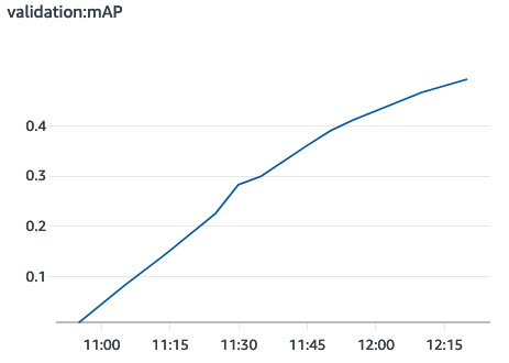
   Figure 5.7 – Validation accuracy

7. We deploy the model to a CPU instance:

   od_predictor = od.deploy(initial_instance_count = 1,                          instance_type = 'ml.c5.2xlarge')

8. We download a test image, and send it for prediction as a byte array. The content type is set to image/jpeg:

   import json

   !wget -O test.jpg https://upload.wikimedia.org/wikipedia/commons/6/67/Chin_Village.jpg

   with open(file_name, 'rb') as image:    f = image.read()    b = bytearray(f)

   od_predictor.content_type = 'image/jpeg'results = od_predictor.predict(b)response = json.loads(results)print(response)

9. The response contains a list of predictions. Each individual prediction contains a class identifier, the confidence score, and the relative coordinates of the bounding box. Here are the first predictions in the response:

   {'prediction': [[14.0, 0.7515302300453186, 0.39770469069480896, 0.37605002522468567, 0.5998836755752563, 1.0], [14.0, 0.6490200161933899, 0.8020403385162354, 0.2027685046195984, 0.9918708801269531, 0.8575668931007385]

   Using this information, we could plot the bounding boxes on the source image. For the sake of brevity, I will not include the code here, but you'll find it in the GitHub repository for this book. The following output shows the result:

   

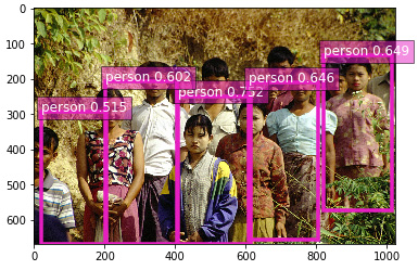
   Figure 5.8 – Test image

10. When we're done, we delete the endpoint as follows:

    od_predictor.delete_endpoint()

This concludes our exploration of object detection. We have one more algorithm to go: semantic segmentation.

Training a semantic segmentation model

In this example, we'll use the semantic segmentation algorithm to build a model on the Pascal VOC dataset that we prepared in a previous section:

1. As usual, we define the data paths, as follows:

   import sagemaker

   session = sagemaker.Session()bucket = sess.default_bucket()  prefix = 'pascalvoc-segmentation'

   s3_train_data = 's3://{}/{}/input/train'.format(bucket, prefix)

   s3_validation_data = 's3://{}/{}/input/validation'.format(bucket, prefix)

   s3_train_annotation_data = 's3://{}/{}/input/train_annotation'.format(bucket, prefix)

   s3_validation_annotation_data = 's3://{}/{}/input/validation_annotation'.format(bucket, prefix)

   s3_output_location = 's3://{}/{}/output'.format(bucket, prefix)

2. We select the semantic segmentation algorithm, and we configure the Estimator function:

   from sagemaker import image_uris

   container = image_uris.retrieve('semantic-segmentation', region)

   seg = sagemaker.estimator.Estimator(          container,          sagemaker.get_execution_role(),          instance_count = 1,          instance_type = 'ml.p3.2xlarge',          output_path = s3_output_location)

3. We define the required hyperparameters. We select a pretrained ResNet-50 network for the base network, and a pretrained FCN for detection. We set the number of classes and training samples. Again, we settle on 30 epochs, which should be enough to start seeing results:

   seg.set_hyperparameters(backbone='resnet-50',                        algorithm='fcn',                        use_pretrained_model=True,                        num_classes=21,                        num_training_samples=1464,                        epochs=30)

4. We configure the four channels, setting the content type to image/jpeg for source images, and image/png for mask images. Then, we launch the training job:

   from sagemaker import TrainingInput

   train_data = TrainingInput(             s3_train_data,              distribution='FullyReplicated',             content_type='image/jpeg',              s3_data_type='S3Prefix')

   validation_data = TrainingInput(                  s3_validation_data,                   distribution='FullyReplicated',                  content_type='image/jpeg',                   s3_data_type='S3Prefix')

   train_annotation = TrainingInput(                   s3_train_annotation_data,                   distribution='FullyReplicated',                   content_type='image/png',                    s3_data_type='S3Prefix')

   validation_annotation = TrainingInput(                        s3_validation_annotation_data,                        distribution='FullyReplicated',                        content_type='image/png',                         s3_data_type='S3Prefix')

   data_channels = {  'train': train_data,  'validation': validation_data,  'train_annotation': train_annotation,  'validation_annotation':validation_annotation }

   seg.fit(inputs=data_channels)

5. Training lasts about 40 minutes. We get a mean intersection-over-union metric (mIOU) of 0.49, as shown in the following plot taken from CloudWatch:
   

   Figure 5.9 – Validation mIOU

6. We deploy the model to a CPU instance:

   seg_predictor = seg.deploy(initial_instance_count=1,                            instance_type='ml.c5.2xlarge')

7. Once the endpoint is in service, we grab a test image, and we send it for prediction as a byte array with the appropriate content type:

   !wget -O test.jpg https://upload.wikimedia.org/wikipedia/commons/e/ea/SilverMorgan.jpg

   filename = 'test.jpg'

   seg_predictor.content_type = 'image/jpeg'seg_predictor.accept = 'image/png'

   with open(filename, 'rb') as image:    img = image.read()    img = bytearray(img)

   response = seg_predictor.predict(img)

8. Using the Python Imaging Library (PIL), we process the response mask and display it:

   import PIL from PIL import Image import numpy as np import io

   num_classes = 21 mask = np.array(Image.open(io.BytesIO(response)))plt.imshow(mask, vmin=0, vmax=num_classes-1, cmap='gray_r')plt.show()

   The following images show the source image and the predicted mask. This result is promising, and would improve with more training:

   

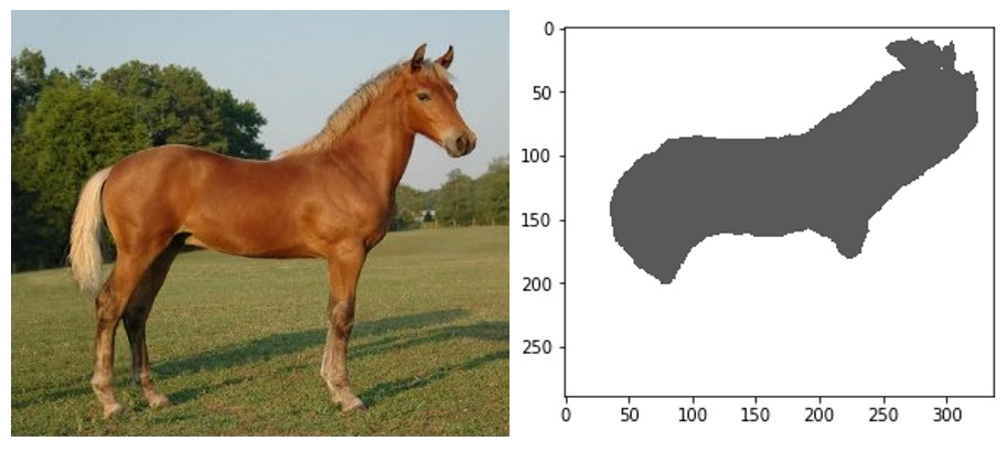
   Figure 5.10 – Test image and segmented test image

9. Predicting again with the protobuf accept type, we receive class probabilities for all the pixels in the source image. The response is a protobuf buffer, which we save to a binary file:

   seg_predictor.content_type = 'image/jpeg'seg_predictor.accept = 'application/x-protobuf'response = seg_predictor.predict(img)

   results_file = 'results.rec'with open(results_file, 'wb') as f:    f.write(response)

10. The buffer contains two tensors: one with the shape of the probability tensor, and one with the actual probabilities. We load them using Apache MXNet and print their shape as follows:

    from sagemaker.amazon.record_pb2 import Record import mxnet as mx

    rec = Record()recordio = mx.recordio.MXRecordIO(results_file, 'r')protobuf = rec.ParseFromString(recordio.read())

    shape = list(rec.features["shape"].int32_tensor.values)values = list(rec.features["target"].float32_tensor.values)

    print(shape.shape)print(values.shape)

    The output is as follows:

    [1, 21, 289, 337]2045253

    This tells us that the values tensor describes one image of size 289x337, where each pixel is assigned 21 probabilities, one for each of the Pascal VOC classes.You can check that 289*337*21=2,045,253.

11. Knowing that, we can now reshape the values tensor, retrieve the 21 probabilities for the (0,0) pixel, and print the class identifier with the highest probability:

    mask = np.reshape(np.array(values), shape)pixel_probs = mask[0,:,0,0]print(pixel_probs)print(np.argmax(pixel_probs))

    Here is the output:

    [9.68291104e-01 3.72813665e-04 8.14868137e-04 1.22414716e-03

    4.57380433e-04 9.95167647e-04 4.29908326e-03 7.52388616e-04

    1.46311778e-03 2.03254796e-03 9.60668200e-04 1.51833100e-03

    9.39570891e-04 1.49350625e-03 1.51627266e-03 3.63648031e-03

    2.17934581e-03 7.69103528e-04 3.05095245e-03 2.10589729e-03

    1.12741732e-03]

    0

    The highest probability is at index 0: the predicted class for pixel (0,0) is class 0, the background class.

12. When we're done, we delete the endpoint as follows:

    seg_predictor.delete_endpoint()

Summary

As you can see, these three algorithms make it easy to train CV models. Even with default hyperparameters, we get good results pretty quickly. Still, we start feeling the need to scale our training jobs. Don't worry: once the relevant features have been covered in future chapters, we'll revisit some of our CV examples and we'll scale them radically!

In this chapter, you learned about the image classification, object detection, and semantic segmentation algorithms. You also learned how to prepare datasets in image, RecordIO, and SageMaker Ground Truth formats. Labeling and preparing data is a critical step that takes a lot of work, and we covered it in great detail. Finally, you learned how to use the SageMaker SDK to train and deploy models with the three algorithms, as well as how to interpret results.

In the next chapter, you will learn how to use built-in algorithms for natural language processing.