Chapter 6: Training Natural Language Processing Models

In the previous chapter, you learned how to use SageMaker's built-in algorithms for Computer Vision (CV) to solve problems including image classification, object detection, and semantic segmentation.

Natural Language Processing (NLP) is another very promising field in machine learning. Indeed, NLP algorithms have proven very effective in modeling language and extracting context from unstructured text. Thanks to this, applications such as search, translation, and chatbots are now commonplace.

In this chapter, you will learn about built-in algorithms designed specifically for NLP tasks. We'll discuss the types of problems that you can solve with them. As in the previous chapter, we'll also cover in great detail how to prepare real-life datasets such as Amazon customer reviews. Of course, we'll train and deploy models too. We will cover all of this under the following topics:

• Discovering the NLP algorithms in Amazon SageMaker
• Preparing natural language datasets
• Using the built-in CV algorithms of BlazingText, Latent Dirichlet Allocation, and Neural Topic Model

Technical requirements

You will need an AWS account to run the examples included in this chapter. If you haven't got one already, please point your browser to https://aws.amazon.com/getting-started/ to create it. You should also familiarize yourself with the AWS Free Tier (https://aws.amazon.com/free/), which lets you use many AWS services for free within certain usage limits.

You will need to install and configure the AWS Command-Line Interface (CLI) for your account (https://aws.amazon.com/cli/).

You will need a working Python 3.x environment. Be careful to not use Python 2.7, as it is no longer maintained. Installing the Anaconda distribution (https://www.anaconda.com/) is not mandatory, but strongly encouraged, as it includes many projects that we will need (Jupyter, pandas, numpy, and more).

The code examples included in the book are available on GitHub at https://github.com/PacktPublishing/Learn-Amazon-SageMaker. You will need to install a Git client to access them (https://git-scm.com/).

Discovering the NLP built-in algorithms in Amazon SageMaker

SageMaker includes four NLP algorithms, enabling supervised and unsupervised learning scenarios. In this section, you'll learn about these algorithms, what kind of problems they solve, and what their training scenarios are:

• BlazingText builds text classification models (supervised learning)or computes word vectors (unsupervised learning). BlazingText is an Amazon-invented algorithm.
• Latent Dirichlet Allocation (LDA) builds unsupervised learning models that group a collection of text documents into topics. This technique is called topic modeling.
• Neural Topic Model (NTM) is another topic modeling algorithm based on neural networks, and it gives you more insight into how topics are built.
• Sequence-to-sequence (seq2seq) builds deep learning models predicting a sequence of output tokens from a sequence of input tokens.

Discovering the BlazingText algorithm

The BlazingText algorithm was invented by Amazon. You can read more about it at https://www.researchgate.net/publication/320760204_BlazingText_Scaling_and_Accelerating_Word2Vec_using_Multiple_GPUs. BlazingText is an evolution of FastText, a library for efficient text classification and representation learning developed by Facebook (https://fasttext.cc).

It lets you train text classification models, as well as compute word vectors. Also called embeddings, word vectors are the cornerstone of many NLP tasks, such as finding word similarities, word analogies, and so on. Word2Vec is one of the leading algorithms to compute these vectors (https://arxiv.org/abs/1301.3781), and it's the one BlazingText implements.

The main improvement of BlazingText is its ability to train on GPU instances, where as FastText only supports CPU instances.

The speed gain is significant, and this is where its name comes from: "blazing" is faster than "fast"! If you're curious about benchmarks, you'll certainly enjoy this blog post: https://aws.amazon.com/blogs/machine-learning/amazon-sagemaker-blazingtext-parallelizing-word2vec-on-multiple-cpus-or-gpus/.

Finally, BlazingText is fully compatible with FastText. Models can be very easily exported and tested, as you will see later in the chapter.

Discovering the LDA algorithm

This unsupervised learning algorithm uses a generative technique, named topic modeling, to identify topics present in a large collection of text documents.It was first applied to machine learning in 2003 (http://jmlr.csail.mit.edu/papers/v3/blei03a.html).

Please note that LDA is not a classification algorithm. You pass it the number of topics to build, not the list of topics you expect. To paraphrase Forrest Gump: "Topic modeling is like a box of chocolates, you never know what you're gonna get."

LDA assumes that every text document in the collection was generated from several latent (meaning "hidden") topics. A topic is represented by a word probability distribution. For each word present in the collection of documents, this distribution gives the probability that the word appears in documents generated by this topic. For example, in a "finance" topic, the distribution would yield high probabilities for words such as "revenue", "quarter", or "earnings", and low probabilities for "ballista" or "platypus" (or so I should think).

Topic distributions are not considered independently. They are represented by a Dirichlet distribution, a multivariate generalization of univariate distributions (https://en.wikipedia.org/wiki/Dirichlet_distribution). This mathematical object gives the algorithm its name.

Given the number of words in the vocabulary and the number of latent topics, the purpose of the LDA algorithm is to build a model that is as close as possible to an ideal Dirichlet distribution. In other words, it will try to group words so that distributions are as well formed as possible, and match the specified number of topics.

Training data needs to be carefully prepared. Each document needs to be converted to a bag of words representation: each word is replaced by a pair of integers, representing a unique word identifier and the word count in the document. The resulting dataset can be saved either to CSV format, or to RecordIO-wrapped protobuf format, a technique we already studied with Factorization machines in Chapter 4, Training Machine Learning Models.

Once the model has been trained, we can score any document, and get a score per topic. The expectation is that documents containing similar words should have similar scores, making it possible to identify their top topics.

Discovering the NTM algorithm

NTM is another algorithm for topic modeling. It was invented by Amazon, and you can read more about it at https://arxiv.org/abs/1511.06038. This blog post also sums up the key elements of the paper:

https://aws.amazon.com/blogs/machine-learning/amazon-sagemaker-neural-topic-model-now-supports-auxiliary-vocabulary-channel-new-topic-evaluation-metrics-and-training-subsampling/

As with LDA, documents need to be converted to a bag-of-words representation, and the dataset can be saved either to CSV or to RecordIO-wrapped protobuf format.

For training, NTM uses a completely different approach based on neural networks, and more precisely, on an encoder architecture (https://en.wikipedia.org/wiki/Autoencoder). In true deep learning fashion, the encoder trains on mini-batches of documents. It tries to learn their latent features by adjusting network parameters through backpropagation and optimization.

Unlike LDA, NTM can tell us which words are the most impactful in each topic. It also gives us two per-topic metrics, Word Embedding Topic Coherence and
Topic Uniqueness:

• WETC tells us how semantically close the topic words are. This value is between 0 and 1, the higher the better. It's computed using the cosine similarity (https://en.wikipedia.org/wiki/Cosine_similarity) of the corresponding word vectors in a pretrained GloVe model (another algorithm similar to Word2Vec).
• TU tells us how unique the topic is, that is to say, whether its words are found in other topics or not. Again, the value is between 0 and 1, and the higher the score, the more unique the topic is.

Once the model has been trained, we can score documents, and get a score per topic.

Discovering the seq2seq algorithm

The seq2seq algorithm is based on Long Short-Term Memory (LSTM) neural networks (https://arxiv.org/abs/1409.3215). As its name implies, seq2seq can be trained to map one sequence of tokens to another. Its main application is machine translation, training on large bilingual corpuses of text, such as the Workshop on Statistical Machine Translation (WMT) datasets (http://www.statmt.org/wmt20/).

In addition to the implementation available in SageMaker, AWS has also packaged the AWS Sockeye (https://github.com/awslabs/sockeye) algorithm into an open source project, which also includes tools for dataset preparation.

I won't cover seq2seq in this chapter. It would take too many pages to get into the appropriate level of detail, and there's no point in just repeating what's already available in the Sockeye documentation.

You can find a seq2seq example in the notebook available at https://github.com/awslabs/amazon-sagemaker-examples/tree/master/introduction_to_amazon_algorithms/seq2seq_translation_en-de. Unfortunately, it uses the low-level boto3 API – which we will cover in Chapter 12, Automating Machine Learning Workflows. Still, it's a valuable read, and you won't have much trouble figuring things out.

Training with NLP algorithms

Just like for CV algorithms, training is the easy part, especially with the SageMaker SDK. By now, you should be familiar with the workflow and the APIs, and we'll keep using them in this chapter.

Preparing data for NLP algorithms is another story. First, real-life datasets are generally pretty bulky. In this chapter, we'll work with millions of samples and hundreds of millions of words. Of course, they need to be cleaned, processed, and converted to the format expected by the algorithm.

As we go through the chapter, we'll use the following techniques:

• Loading and cleaning data with the pandas library (https://pandas.pydata.org)
• Removing stop words and lemmatizing with the Natural Language Toolkit (NLTK) library (https://www.nltk.org)
• Tokenizing with the spacy library (https://spacy.io/)
• Building vocabularies and generating bag-of-words representations with the gensim library (https://radimrehurek.com/gensim/)
• Running data processing jobs with Amazon SageMaker Processing, which we studied in Chapter 2, Handling Data Preparation Techniques

Granted, this isn't an NLP book, and we won't go extremely far into processing data. Still, this will be quite fun, and hopefully an opportunity to learn about popular open source tools for NLP.

Preparing natural language datasets

For the CV algorithms in the previous chapter, data preparation focused on the technical format required for the dataset (Image format, RecordIO, or augmented manifest). The images themselves weren't processed.

Things are quite different for NLP algorithms. Text needs to be heavily processed, converted, and saved in the right format. In most learning resources, these steps are abbreviated or even ignored. Data is already "automagically" ready for training, leaving the reader frustrated and sometimes dumbfounded on how to prepare their own datasets.

No such thing here! In this section, you'll learn how to prepare NLP datasets in different formats. Once again, get ready to learn a lot!

Let's start with preparing data for BlazingText.

Preparing data for classification with BlazingText

BlazingText expects labeled input data in the same format as FastText:

• A plain text file, with one sample per line.
• Each line has two fields:

  a) A label in the form of __label__LABELNAME__

  b) The text itself, formed into space-separated tokens (words and punctuations)

Let's get to work and prepare a customer review dataset for sentiment analysis (positive, neutral, or negative). We'll use the Amazon Reviews dataset available at https://s3.amazonaws.com/amazon-reviews-pds/readme.html. That should be more than enough real-life data.

Before starting, please make sure that you have enough storage space. Here, I'm using a notebook instance with 10 GB of storage. I've also picked a C5 instance type to run processing steps faster:

1. Let's download the camera reviews:

   %%sh

   aws s3 cp s3://amazon-reviews-pds/tsv/amazon_reviews_us_Camera_v1_00.tsv.gz /tmp

2. We load the data with pandas, ignoring any line that causes an error. We also drop any line with missing values:

   data = pd.read_csv(    '/tmp/amazon_reviews_us_Camera_v1_00.tsv.gz',     sep=' ', compression='gzip',     error_bad_lines=False, dtype='str')

   data.dropna(inplace=True)

3. We print the data shape and the column names:

   print(data.shape)print(data.columns)

   This gives us the following output:

   (1800755, 15)

   Index(['marketplace','customer_id','review_id','product_id','product_parent', 'product_title','product_category',  'star_rating','helpful_votes','total_votes','vine', 'verified_purchase','review_headline','review_body', 'review_date'], dtype='object')

4. 1.8 million lines! We keep 100,000, which is enough for our purpose. We also drop all columns except star_rating and review_body:

   data = data[:100000]data = data[['star_rating', 'review_body']]

5. Based on star ratings, we add a new column named label, with labels in the proper format. You have to love how pandas makes this so simple. Then, we drop the star_rating column:

   data['label'] = data.star_rating.map({    '1': '__label__negative__',    '2': '__label__negative__',    '3': '__label__neutral__',    '4': '__label__positive__',    '5': '__label__positive__'})

   data = data.drop(['star_rating'], axis=1)

6. BlazingText expect labels at the beginning of each line, so we move the label column to the front:

   data = data[['label', 'review_body']]

7. Data should now look like in the following figure:
   

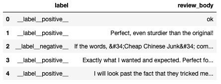
   Figure 6.1 – Viewing the dataset

8. BlazingText expects space-separated tokens: each word and each punctuation sign must be space-separated from the next. Let's use the handy punkt tokenizer from the nltk library. Depending on the instance type you're using, this could take a couple of minutes:

   !pip -q install nltk import nltk nltk.download('punkt')

   data['review_body'] = data['review_body'].apply(nltk.word_tokenize)

9. We join tokens into a single string, which we also convert to lower case:

   data['review_body'] = data.apply(lambda row: " ".join(row['review_body']).lower(), axis=1)

10. The data should now look like that in the following figure. Notice that all the tokens are correctly space-separated:
    

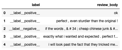
    Figure 6.2 – Viewing the tokenized dataset

11. Finally, we split the dataset for training (95%) and validation (5%), and we save both splits as plain text files:

    from sklearn.model_selection import train_test_split

    training, validation = train_test_split(data, test_size=0.05)

    np.savetxt('/tmp/training.txt', training.values, fmt='%s')np.savetxt('/tmp/validation.txt', validation.values, fmt='%s')

12. If you open one of the files, you should see plenty of lines similar to this one:

    __label__neutral__ really works for me , especially on the streets of europe . wished it was less expensive though . the rain cover at the base really works . the padding which comes in contact with your back though will suffocate & make your back sweaty .

Data preparation wasn't too bad, was it? Still, tokenization ran for a minute or two. Now, imagine running it on millions of samples. Sure, you could fire up a larger Notebook instance or use a larger environment in SageMaker Studio. You'd also pay more for as long as you're using it, which would probably be wasteful if only this one step required that extra computing muscle. In addition, imagine having to run the same script on many other datasets. Do you want to do this manually again and again, waiting 20 minutes every time and hoping Jupyter doesn't crash? Certainly not, I should think!

You already know the answer to both problems. It's Amazon SageMaker Processing, which we studied in Chapter 2, Handling Data Preparation Techniques. You should have the best of both worlds, using the smallest and least expensive environment possible for experimentation, and running on-demand jobs when you need more resources. Day in, day out, you'll save money and get the job done faster.

Let's move this processing code to SageMaker Processing.

Preparing data for classification with BlazingText, version 2

We've covered this in detail in Chapter 2, Handling Data Preparation Techniques, so I'll go faster this time:

1. We upload the dataset to S3:

   import sagemaker

   session = sagemaker.Session()prefix = 'amazon-reviews-camera'

   input_data = session.upload_data(    path='/tmp/amazon_reviews_us_Camera_v1_00.tsv.gz',     key_prefix=prefix)

2. We define the processor:

   from sagemaker.sklearn.processing import SKLearnProcessor

   sklearn_processor = SKLearnProcessor(   framework_version='0.20.0',   role= sagemaker.get_execution_role(),   instance_type='ml.c5.2xlarge',   instance_count=1)

3. We run the processing job, passing the processing script and its arguments:

   from sagemaker.processing import ProcessingInput, ProcessingOutput

   sklearn_processor.run(    code='preprocessing.py',

       inputs=[        ProcessingInput(            source=input_data,            destination='/opt/ml/processing/input')    ],    outputs=[        ProcessingOutput(            output_name='train_data',            source='/opt/ml/processing/train'),        ProcessingOutput(            output_name='validation_data',            source='/opt/ml/processing/validation')    ],    arguments=[        '--filename',             'amazon_reviews_us_Camera_v1_00.tsv.gz',        '--num-reviews', '100000',        '--split-ratio', '0.05'    ])

4. The abbreviated preprocessing script is as follows. The full version is in the GitHub repository for the book. We first install the nltk package:

   import argparse, os, subprocess, sys import pandas as pd import numpy as np from sklearn.model_selection import train_test_split

   def install(package):    subprocess.call([sys.executable, "-m", "pip",                     "install", package])

   if __name__=='__main__':    install('nltk')    import nltk

5. We read the command-line arguments:

       parser = argparse.ArgumentParser()    parser.add_argument('--filename', type=str)    parser.add_argument('--num-reviews', type=int)    parser.add_argument('--split-ratio', type=float,                         default=0.1)

       args, _ = parser.parse_known_args()    filename = args.filename     num_reviews = args.num_reviews     split_ratio = args.split_ratio

6. We read the input dataset and process it as follows:

       input_data_path =     os.path.join('/opt/ml/processing/input', filename)

       data = pd.read_csv(input_data_path, sep=' ',            compression='gzip', error_bad_lines=False,           dtype='str')

       # Process data     . . .

7. Finally, we split it for training and validation, and save it to two text files:

       training, validation = train_test_split(                           data, test_size=split_ratio)

       training_output_path = os.path.join('                              /opt/ml/processing/train',                              'training.txt')    

       validation_output_path = os.path.join(                          /opt/ml/processing/validation',                          'validation. txt')

       np.savetxt(training_output_path,                training.values, fmt='%s')

       np.savetxt(validation_output_path,                validation.values, fmt='%s')

As you can see, it doesn't take much to convert manual processing code to a SageMaker Processing job. You can actually reuse most of the code too, as it deals with generic topics such as command-line arguments, inputs, and outputs. The only trick is using subprocess.call to install dependencies inside the processing container.

Equipped with this script, you can now process data at scale as often as you want, without having to run and manage long-lasting notebooks.

Now, let's prepare data for the other BlazingText scenario: word vectors!

Preparing data for word vectors with BlazingText

BlazingText lets you compute word vectors easily and at scale. It expects input data in the following format:

• A plain text file, with one sample per line.
• Each sample must have space-separated tokens (words and punctuations).

Let's process the same dataset as in the previous section:

1. We'll need the spacy library, so let's install it along with its English language model:

   %%sh pip -q install spacy python -m spacy download en

2. We load the data with pandas, ignoring any line that causes an error. We also drop any line with missing values. We should have more than enough data anyway:

   data = pd.read_csv(    '/tmp/amazon_reviews_us_Camera_v1_00.tsv.gz',     sep=' ', compression='gzip',     error_bad_lines=False, dtype='str')

   data.dropna(inplace=True)

3. We keep 100,000 lines, and we also drop all columns except review_body:

   data = data[:100000]data = data[['review_body']]

   We write a function to tokenize reviews with spacy, and we apply it to the DataFrame. This step should be noticeably faster than nltk tokenization in the previous example, as spacy is based on Cython (https://cython.org):

   import spacy

   spacy_nlp = spacy.load('en')

   def tokenize(text):    tokens = spacy_nlp.tokenizer(text)    tokens = [ t.text for t in tokens ]    return " ".join(tokens).lower()

   data['review_body'] = data['review_body'].apply(tokenize)

4. The data should now look like that in the following figure:
   

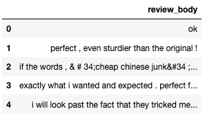
   Figure 6.3 – Viewing the tokenized dataset

5. Finally, we save the reviews to a plain text file:

   import numpy as np np.savetxt('/tmp/training.txt', data.values, fmt='%s')

6. Opening this file, you should see one tokenized review per line:

   Ok perfect , even sturdier than the original !

Here too, we should really be running these steps using SageMaker Processing. You'll find the corresponding notebook and preprocessing script in the GitHub repository for the book.

Now, let's prepare data for the LDA and NTM algorithms.

Preparing data for topic modeling with LDA and NTM

In this example, we will use the Million News Headlines dataset (https://doi.org/10.7910/DVN/SYBGZL), which is also available in the GitHub repository. As the name implies, it contains a million news headlines from Australian news source ABC. Unlike product reviews, headlines are very short sentences. Building a topic model should be an interesting challenge!

Tokenizing data

As you would expect, both algorithms require a tokenized dataset:

1. We'll need the nltk and the gensim libraries, so let's install them:

   %%sh pip -q install nltk gensim

2. Once we've downloaded the dataset, we load it entirely with pandas:

   num_lines = 1000000 data = pd.read_csv('abcnews-date-text.csv.gz',                    compression='gzip',                    error_bad_lines=False,                    dtype='str', nrows=num_lines)

3. The data should look like that in the following figure:
   

   Figure 6.4 – Viewing the tokenized dataset

4. It's sorted by date, and we shuffle it as a precaution. We then drop the date column:

   data = data.sample(frac=1)data = data.drop(['publish_date'], axis=1)

5. We write a function to clean up and process the headlines. First, we get rid of all punctuation signs and digits. Using nltk, we also remove stop words, namely words that are extremely common and don't add any context, such as this, any, and so on. In order to reduce the vocabulary size while keeping the context, we could apply either stemming or lemmatisation, two popular NLP techniques (https://nlp.stanford.edu/IR-book/html/htmledition/stemming-and-lemmatization-1.html).

   Let's go with the latter here. Depending on your instance type, this could run for several minutes:

   import string import nltk from nltk.corpus import stopwords #from nltk.stem.snowball import SnowballStemmer from nltk.stem import WordNetLemmatizer

   nltk.download('stopwords')stop_words = stopwords.words('english')

   #stemmer = SnowballStemmer("english")wnl = WordNetLemmatizer()

   def process_text(text):    for p in string.punctuation:        text = text.replace(p, '')        text = ''.join([c for c in text if not                        c.isdigit()])        text = text.lower().split()        text = [w for w in text if not w in stop_words]        #text = [stemmer.stem(w) for w in text]        text = [wnl.lemmatize(w) for w in text]        return text

   data['headline_text'] = data['headline_text'].apply(process_text)

6. Once processed, the data should look like that in the following figure:

Figure 6.5 – Viewing the lemmatized dataset

Now that reviews have been tokenized, we need to convert them to a bag-of-words representation, replacing each word with a unique integer identifier and its frequency count.

Converting data to bag of words

We will convert the reviews into a bag of words using the following steps:

1. The gensim library has exactly what we need! We build a dictionary, the list of all words present in the document collection:

   from gensim import corpora

   dictionary = corpora.Dictionary(data['headline_text'])print(dictionary)

   The dictionary looks like this:

   Dictionary(83131 unique tokens: ['aba', 'broadcasting', 'community', 'decides', 'licence']...)

   This number feels very high. If we have too many dimensions, training will be very long, and the algorithm may have trouble fitting the data. For example, NTM is based on a neural network architecture. The input layer will be sized based on the number of tokens, so we need to keep them reasonably low. It will speed up training, and help the encoder learn a manageable number of latent features.

2. We could go back and clean headlines some more. Instead, we use a gensim function that removes extreme words, outlier words that are either extremely rare or extremely frequent. Then, taking a bold bet, we decide to restrict the vocabulary to the top 512 remaining words. Yes, that's less than 1%:

   dictionary.filter_extremes(keep_n=512)

3. We write the vocabulary to a text file. Not only does this help us check what the top words are, but we'll also pass this file to the NTM algorithm as an extra channel. You'll see why this is important when we train the model:

   with open('vocab.txt', 'w') as f:    for index in range(0,len(dictionary)):        f.write(dictionary.get(index)+' ')

4. We use the dictionary to build a bag of words for each headline. It's stored in a new column called tokens. When we're done, we drop the text review:

   data['tokens'] = data.apply(lambda row: dictionary.doc2bow(row['headline_text']), axis=1)

   data = data.drop(['headline_text'], axis=1)

5. The data should now look like that in the following figure:

Figure 6.6 – Viewing the bag-of-words dataset

As you can see, each word has been replaced with its unique identifier and its frequency count in the review. For instance, the last line tells us that word #11 is present once, word #12 is present once, and so on.

Data processing is now complete. The last step is to save it to the appropriate input format.

Saving input data

NTM and LDA expect data in either the CSV format, or the RecordIO-wrapped protobuf format. Just like for the Factorization matrix example in Chapter 4, Training Machine Learning Models, the data we're working with is quite sparse. Any given review only contains a small number of words from the vocabulary. As CSV is a dense format,we would end up with a huge amount of zero-frequency words. Not a good idea!

Once again, we'll use lil_matrix, a sparse matrix object available in SciPy.It will have as many lines as we have reviews and as many columns as we have words in the dictionary:

1. We create the sparse matrix as follows:

   from scipy.sparse import lil_matrix

   num_lines = data.shape[0]num_columns = len(dictionary)token_matrix = lil_matrix((num_lines,num_columns))               .astype('float32')

2. We write a function to add a headline to the matrix. For each token, we simply write its frequency in the appropriate column:

   def add_row_to_matrix(line, row):    for token_id, token_count in row['tokens']:        token_matrix[line, token_id] = token_count     return

3. We then iterate over headlines and add them to the matrix. Quick note: we can't use row index values, as they might be larger than the number of lines:

   line = 0 for _, row in data.iterrows():    add_row_to_matrix(line, row)    line+=1

4. The last step is to write this matrix into a memory buffer in protobuf format and upload it to S3 for future use:

   import io, boto3 import sagemaker import sagemaker.amazon.common as smac

   buf = io.BytesIO()smac.write_spmatrix_to_sparse_tensor(buf, token_matrix, None)buf.seek(0)

   bucket = sagemaker.Session().default_bucket()prefix = 'headlines-lda-ntm'train_key = 'reviews.protobuf'obj = '{}/{}'.format(prefix, train_key))

   s3 = boto3.resource('s3')s3.Bucket(bucket).Object(obj).upload_fileobj(buf)s3_train_path = 's3://{}/{}'.format(bucket,obj)

5. Building the (1000000, 512) matrix takes a few minutes. Once it's been uploaded to S3, we can see that it's only 42 MB. Lil' matrix indeed:

   $ aws s3 ls s3://sagemaker-eu-west-1-123456789012/amazon-reviews-ntm/training.protobuf

   43884300 training.protobuf

This concludes data preparation for LDA and NTM. Now, let's see how we can use text datasets prepared with SageMaker Ground Truth.

Using datasets labeled with SageMaker Ground Truth

As discussed in Chapter 2, Handling Data Preparation Techniques, SageMaker Ground Truth supports text classification tasks. We could definitely use their output to build a dataset for FastText or BlazingText.

First, I ran a quick text classification job on a few sentences, applying one of two labels: "aws_service" if the sentence mentions an AWS service, "no_aws_service"if it doesn't.

Once the job is complete, I can fetch the augmented manifest from S3. It's in JSON Lines format, and here's one of its entries:

{"source":"With great power come great responsibility. The second you create AWS resources, you're responsible for them: security of course, but also cost and scaling. This makes monitoring and alerting all the more important, which is why we built services like Amazon CloudWatch, AWS Config and AWS Systems Manager.","my-text-classification-job":0,"my-text-classification-job-metadata":{"confidence":0.84,"job-name":"labeling-job/my-text-classification-job","class-name":"aws_service","human-annotated":"yes","creation-date":"2020-05-11T12:44:50.620065","type":"groundtruth/text-classification"}}

Shall we write a bit of Python code to put this in BlazingText format? Of course!

1. We load the augmented manifest directly from S3:

   import pandas as pd

   bucket = 'sagemaker-book'prefix = 'chapter2/classif/output/my-text-classification-job/manifests/output'manifest = 's3://{}/{}/output.manifest'.format(bucket, prefix)

   data = pd.read_json(manifest, lines=True)

   The data looks like that in the following figure:

   

   Figure 6.7 – Viewing the labeled dataset

2. The label is buried in the "my-text-classification-job-metadata" column. We extract it into a new column:

   def get_label(metadata):    return metadata['class-name']

   data['label'] = data['my-text-classification-job-metadata'].apply(get_label)

   data = data[['label', 'source']]

   The data now looks like that in the following figure. From then on, we can apply tokenization, and so on. That was easy, wasn't it?

Figure 6.8 – Viewing the processed dataset

Now let's build NLP models!

Using the built-in algorithms for NLP

In this section, we're going to train and deploy models with BlazingText, LDA, and NTM. Of course, we'll use the datasets prepared in the previous section.

Classifying text with BlazingText

BlazingText makes it extremely easy to build a text classification model, especially if you have no NLP skills. Let's see how:

1. We upload the training and validation datasets to S3. Alternatively, we could use the output paths returned by a SageMaker Processing job:

   import boto3, sagemaker

   session = sagemaker.Session()bucket = session.default_bucket()prefix = 'amazon-reviews'

   s3_train_path = session.upload_data(path='/tmp/training.txt', bucket=bucket, key_prefix=prefix+'/input/train')

   s3_val_path = session.upload_data(path='/tmp/validation.txt', bucket=bucket, key_prefix=prefix+'/input/validation')

   s3_output = 's3://{}/{}/output/'.format(bucket, prefix)

2. We configure the Estimator function for BlazingText:

   from sagemaker import image_uris region_name = boto3.Session().region_name container = image_uris.retrieve('blazingtext', region)

   bt = sagemaker.estimator.Estimator(container,      sagemaker.get_execution_role(),     instance_count=1,     instance_type='ml.g4dn.xlarge',     output_path=s3_output)

3. We set a single hyperparameter, telling BlazingText to train in supervised mode:

   bt.set_hyperparameters(mode='supervised')

4. We define channels, setting the content type to text/plain, and then we launch the training:

   from sagemaker import TrainingInput

   train_data = TrainingInput (s3_train_path, distribution='FullyReplicated', content_type='text/plain', s3_data_type='S3Prefix')

   validation_data = TrainingInput (s3_val_path,distribution='FullyReplicated', content_type='text/plain',s3_data_type='S3Prefix')

   s3_channels = {'train': train_data,                'validation': validation_data}

   bt.fit(inputs=s3_channels)

5. We get a validation accuracy close to 88%, which is quite good in the absence of any hyperparameter tweaking. We then deploy the model to a small CPU instance:

   bt_predictor = bt.deploy(initial_instance_count=1,                          instance_type='ml.t2.medium')

6. Once the endpoint is up, we send three tokenized samples for prediction, asking for all three labels:

   import json

   sentences = ['This is a bad camera it doesnt work at all , i want a refund  . ' , 'The camera works , the pictures are decent quality, nothing special to say about it . ' , 'Very happy to have bought this , exactly what I needed . ']

   payload = {"instances":sentences, "configuration":{"k": 3}}

   bt_predictor.content_type = 'application/json'response = bt_predictor.predict(json.dumps(payload))

7. Printing the response, we see that the three samples were correctly categorized. It's interesting to see that the second review is neutral/positive. Indeed, it doesn't include any negative words:

   [{'prob': [0.9758228063583374, 0.023583529517054558, 0.0006236258195713162], 'label': ['__label__negative__', '__label__neutral__', '__label__positive__']}, {'prob': [0.5177792906761169, 0.2864232063293457, 0.19582746922969818], 'label': ['__label__neutral__', '__label__positive__', '__label__negative__']}, {'prob': [0.9997835755348206, 0.000205090589588508, 4.133415131946094e-05], 'label': ['__label__positive__', '__label__neutral__', '__label__negative__']}]

8. As usual, we delete the endpoint once we're done:

   bt_predictor.delete_endpoint()

Now, let's train BlazingText to compute word vectors.

Computing word vectors with BlazingText

The code is almost identical to the previous example, with only two differences. First, there is only one channel, containing training data. Second, we need to set BlazingText to unsupervised learning mode.

BlazingText supports the training modes implemented in Word2Vec: skipgram and continuous bag of words (cbow). It adds a third mode, batch_skipgram, for faster distributed training. It also supports subword embeddings, a technique that makes it possible to return a word vector for words that are misspelled or not part of the vocabulary.

Let's go for skipgram with subword embeddings. We leave the dimension of vectors unchanged (the default is 100):

bt.set_hyperparameters(mode='skipgram', subwords=True)

Unlike other algorithms, there is nothing to deploy here. The model artifact is in S3 and can be used for downstream NLP applications.

Speaking of which, BlazingText is compatible with FastText, so how about trying to load the models we just trained in FastText?

Using BlazingText models with FastText

First, we need to compile FastText, which is extremely simple. You can even do it on a Notebook instance without having to install anything:

$ git clone https://github.com/facebookresearch/fastText.git $ cd fastText $ make

Let's first try our classification model.

Using a BlazingText classification model with FastText

We will try the model using the following steps:

1. We copy the model artifact from S3 and extract it as follows:

   $ aws s3 ls s3://sagemaker-eu-west-1-123456789012/amazon-reviews/output/JOB_NAME/output/model.tar.gz .$ tar xvfz model.tar.gz

2. We load model.bin with FastText:

   $ fasttext predict model.bin -

3. We predict samples and view their top class as follows:

   This is a bad camera it doesnt work at all , i want a refund  .__label__negative__

   The camera works , the pictures are decent quality, nothing special to say about it .__label__neutral__

   Very happy to have bought this , exactly what I needed __label__positive__

We exit with Ctrl + C. Now, let's explore our vectors.

Using BlazingText word vectors with FastText

We will now use FastText with the vectors as follows:

1. We copy the model artifact from S3, and we extract it:

   $ aws s3 ls s3://sagemaker-eu-west-1-123456789012/amazon-reviews-word2vec/output/JOB_NAME/output/model.tar.gz .$ tar xvfz model.tar.gz

2. We can explore word similarities. For example, let's look for words that are closest to telephoto. This could help us improve how we handle search queries or how we recommend similar products:

   $ fasttext nn vectors.bin Query word? Telephoto telephotos 0.951023 75-300mm 0.79659 55-300mm 0.788019 18-300mm 0.782396 . . .

3. We can also look for analogies. For example, let's ask our model the following question: what's the Canon equivalent for the Nikon D3300 camera?

   $ fasttext analogies vectors.bin Query triplet (A - B + C)? nikon d3300 canon xsi 0.748873 700d 0.744358 100d 0.735871

   According to our model, you should consider the XSI and 700d cameras!

As you can see, word vectors are amazing and BlazingText makes it easy to compute them at any scale. Now, let's move on to topic modeling, another fascinating subject.

Modeling topics with LDA

In a previous section, we prepared a million news headlines, and we're now going to use them for topic modeling with LDA:

1. By loading the process from the dataset in S3, we define the useful paths:

   import sagemaker

   session = sagemaker.Session()bucket = session.default_bucket()prefix = reviews-lda-ntm'train_key = 'reviews.protobuf'

   obj = '{}/{}'.format(prefix, train_key)s3_train_path = 's3://{}/{}'.format(bucket,obj)s3_output = 's3://{}/{}/output/'.format(bucket, prefix)

2. We configure the Estimator function:

   from sagemaker import image_uris

   region_name = boto3.Session().region_name container = image_uris.retrieve('lda', region)

   lda = sagemaker.estimator.Estimator(container,       role = sagemaker.get_execution_role(),       instance_count=1,                                      instance_type='ml.c5.2xlarge',       output_path=s3_output)

3. We set hyperparameters: how many topics we want to build (10), how many dimensions the problem has (the vocabulary size), and how many samples we're training on. Optionally, we can set a parameter named alpha0. According to the documentation: "Small values are more likely to generate sparse topic mixtures and large values (greater than 1.0) produce more uniform mixtures". Let's set it to 0.1 and hope that the algorithm can indeed build well-identified topics:

   lda.set_hyperparameters(num_topics=5,   feature_dim=len(dictionary),   mini_batch_size=num_lines,   alpha0=0.1)

4. We launch training. As RecordIO is the default format expected by the algorithm, we don't need to define channels:

   lda.fit(inputs={'train': s3_train_path})

5. Once training is complete, we deploy to a small CPU instance:

   lda_predictor = lda.deploy(initial_instance_count=1,                            instance_type='ml.t2.medium')

6. Before we send samples for prediction, we need to process them just like we processed the training set. We write a function that takes care of this: building a sparse matrix, filling it with bags of words, and saving to an in-memory protobuf buffer:

   def process_samples(samples, dictionary):    num_lines = len(samples)    num_columns = len(dictionary)    sample_matrix = lil_matrix((num_lines,                      num_columns)).astype('float32')

       for line in range(0, num_lines):        s = samples[line]        s = process_text(s)        s = dictionary.doc2bow(s)        for token_id, token_count in s:            sample_matrix[line, token_id] = token_count         line+=1

       buf = io.BytesIO()    smac.write_spmatrix_to_sparse_tensor(buf,                                          sample_matrix,                                          None)    buf.seek(0)    return buf

   Please note that we need the dictionary here. This is why the corresponding SageMaker Processing job saved a pickled version of it, which we could later unpickle and use.

7. Then, we define a Python array containing five headlines, named samples. These are real headlines I copied from the ABC news website at https://www.abc.net.au/news/:

   samples = [ "Major tariffs expected to end Australian barley trade to China", "Satellite imagery sparks more speculation on North Korean leader Kim Jong-un", "Fifty trains out of service as fault forces Adelaide passengers to 'pack like sardines", "Germany's Bundesliga plans its return from lockdown as football world watches", "All AFL players to face COVID-19 testing before training resumes" ]

8. Let's process and predict them:

   lda_predictor.content_type = 'application/x-recordio-protobuf'

   response = lda_predictor.predict(           process_samples(samples, dictionary))print(response)

9. The response contains a score vector for each review (extra decimals have been removed for brevity). Each vector reflects a mix of topics, with a score per topic.All scores add up to 1:

   {'predictions': [{'topic_mixture': [0,0.22,0.54,0.23,0,0,0,0,0,0]}, {'topic_mixture': [0.51,0.49,0,0,0,0,0,0,0,0]}, {'topic_mixture': [0.38,0,0.22,0,0.40,0,0,0,0,0]}, {'topic_mixture': [0.38,0.62,0,0,0,0,0,0,0,0]}, {'topic_mixture': [0,0.75,0,0,0,0,0,0.25,0,0]}]}

10. This isn't easy to read. Let's print the top topic and its score:

    import numpy as np

    vecs = [r['topic_mixture'] for r in response['predictions']]

    for v in vecs:    top_topic = np.argmax(v)    print("topic %s, %2.2f" % (top_topic, v[top_topic]))

    This prints out the following result:

    topic 2, 0.54 topic 0, 0.51 topic 4, 0.40 topic 1, 0.62 topic 1, 0.75

11. As usual, we delete the endpoint once we're done:

    lda_predictor.delete_endpoint()

Interpreting LDA results is not easy, so let's be careful here. No wishful thinking!

• We see that each headline has a definite topic, which is good news. Apparently, LDA was able to identify solid topics, maybe thanks to the low alpha0 value.
• The top topics for unrelated headlines are different, which is promising.
• The last two headlines are both about sports and their top topic is the same, which is another good sign.
• All five reviews scored zero on topics 5, 6, 8, and 9. This probably means that other topics have been built, and we would need to run more examples to discover them.

Is this a successful model? Probably. Can we be confident that topic 0 is about world affairs, topic 1 about sports, and topic 2 about commerce? Not until we've predicted a few thousand more reviews and checked that related headlines are assigned to the same topic.

As mentioned at the beginning of the chapter, LDA is not a classification algorithm.It has a mind of its own and it may build totally unexpected topics. Maybe it will group headlines according to sentiment or city names. It all depends on the distribution of these words inside the document collection.

Wouldn't it be nice if we could see which words "weigh" more in a certain topic?That would certainly help us understand topics a little better. Enter NTM!

Modeling topics with NTM

This example is very similar to the previous one. We'll just highlight the differences, and you'll find a full example in the GitHub repository for the book. Let's get into it:

1. We upload the vocabulary file to S3:

   s3_auxiliary_path = session.upload_data(path='vocab.txt', key_prefix=prefix + '/input/auxiliary')

2. We select the NTM algorithm:

   from sagemaker import image_uris

   region_name = boto3.Session().region_name container = image_uris.retrieve('ntm', region)

3. Once we've configured the Estimator, we set the hyperparameters:

   ntm.set_hyperparameters(num_topics=10,                         feature_dim=len(dictionary),                        optimizer='adam',                        mini_batch_size=256,                        num_patience_epochs=10)

4. We launch training, passing the vocabulary file in the auxiliary channel:

   ntm.fit(inputs={'train': s3_training_path,                 'auxiliary': s3_auxiliary_path})

When training is complete, we see plenty of information in the training log. First, we see the average WETC and TU scores for the 10 topics:

(num_topics:10) [wetc 0.42, tu 0.86]

These are decent results. Topic unicity is high, and the semantic distance between topic words is average.

For each topic, we see its WETC and TU scores, as well as its top words, that is to say, the words that have the highest probability of appearing in documents associated with this topic.

• Let's look at each one in detail and try to put names to topics:
• Topic 0 is pretty obvious, I think. Almost all words are related to crime, so let's call it crime:

  [0.51, 0.84] stabbing charged guilty pleads murder fatal man assault bail jailed alleged shooting arrested teen girl accused boy car found crash

• The following topic, topic 1, is a little fuzzier. How about legal?

  [0.36, 0.85] seeker asylum climate live front hears change export carbon tax court wind challenge told accused rule legal face stand boat

• Topic 2 is about accidents and fires. Let's call it disaster:

  [0.39, 0.78] seeker crew hour asylum cause damage truck country firefighter blaze crash warning ta plane near highway accident one fire fatal

• Topic 3 is obvious: sports. The TU score is the highest, showing that sports articles use a very specific vocabulary found nowhere else:

  [0.54, 0.93] cup world v league one match win title final star live victory england day nrl miss beat team afl player

• Topic 4 is a strange mix of weather information and natural resources. It has the lowest WETC and the lowest TU scores too. Let's call it unknown1:

  [0.35, 0.77] coast korea gold north east central pleads west south guilty queensland found qld rain beach cyclone northern nuclear crop mine

• Topic 5 is about world affairs, it seems. Let's call it international:

  [0.38, 0.88] iraq troop bomb trade korea nuclear kill soldier iraqi blast pm president china pakistan howard visit pacific u abc anti

• Topic 6 feels like local news, as it contains abbreviations for Australian regions: qld is Queensland, ta is Tasmania, nsw is New South Wales, and so on. Let's call it local:

  [0.25, 0.88] news hour country rural national abc ta sport vic abuse sa nsw weather nt club qld award business

• Topic 7 is a no-brainer: finance. It has the highest WETC score, showing that its words are closely related from a semantic point of view. Topic unicity is also very high, and we would probably see the same for domain-specific topics on medicine or engineering:

  [0.62, 0.90] share dollar rise rate market fall profit price interest toll record export bank despite drop loss post high strong trade

• Topic 8 is about politics, with a bit of crime thrown in. Some people would say that's actually the same thing. As we already have a crime topic, we'll name this one politics:

  [0.41, 0.90] issue election vote league hunt interest poll parliament gun investigate opposition raid arrest police candidate victoria house northern crime rate

• Topic 9 is another mixed bag. It's hard to say whether it's about farming or missing people! Let's go with unknown2:

  [0.37, 0.84] missing search crop body found wind rain continues speaks john drought farm farmer smith pacific crew river find mark tourist

All things considered, that's a pretty good model: 8 clear topics out of 10.

Let's define our list of topics and run our sample headlines through the model after deploying it:

topics = ['crime','legal','disaster','sports','unknown1',          'international','local','finance','politics',           'unknown2']

samples = [ "Major tariffs expected to end Australian barley trade to China", "US woman wanted over fatal crash asks for release after coronavirus halts extradition", "Fifty trains out of service as fault forces Adelaide passengers to 'pack like sardines", "Germany's Bundesliga plans its return from lockdown as football world watches", "All AFL players to face COVID-19 testing before training resumes" ]

We use the following function to print the top three topics and their score:

import numpy as np

for r in response['predictions']:    sorted_indexes = np.argsort(r['topic_weights']).tolist()    sorted_indexes.reverse()    top_topics = [topics[i] for i in sorted_indexes]    top_weights = [r['topic_weights'][i]                    for i in sorted_indexes]

    pairs = list(zip(top_topics, top_weights))    print(pairs[:3])

Here's the output:

[('finance', 0.30),('international', 0.22),('sports', 0.09)][('unknown1', 0.19),('legal', 0.15),('politics', 0.14)][('crime', 0.32), ('legal', 0.18), ('international', 0.09)][('sports', 0.28),('unknown1', 0.09),('unknown2', 0.08)][('sports', 0.27),('disaster', 0.12),('crime', 0.11)]

Headlines 0, 2, 3, and 4 are right on target. That's not surprising given how strong these topics are.

Headline 1 scores very high on the topic we called legal. Maybe Adelaide passengers should sue the train company? Seriously, we would need to find other matching headlines to get a better sense of what the topic is really about.

As you can see, NTM makes it easier to understand what topics are about. We could improve the model by processing the vocabulary file, adding or removing specific words to influence topics, increase the number of topics, fiddle with alpha0, and so on.My intuition tells me that we should really see a weather topic in there. Please experiment and see if you want make it appear.

If you'd like to run another example, you'll find interesting techniques in this notebook:

https://github.com/awslabs/amazon-sagemaker-examples/blob/master/introduction_to_applying_machine_learning/ntm_20newsgroups_topic_modeling/ntm_20newsgroups_topic_model.ipynb

Summary

NLP is a very exciting topic. It's also a difficult one because of the complexity of language in general, and due to how much processing is required to build datasets. Having said that, the built-in algorithms in SageMaker will help you get good results out of the box. Training and deploying models are straightforward processes, which leaves you more time to explore, understand, and prepare data.

In this chapter, you learned about the BlazingText, LDA, and NTM algorithms. You also learned how to process datasets using popular open source tools such as nltk, spacy, and gensim, and how to save them in the appropriate format. Finally, you learned how to use the SageMaker SDK to train and deploy models with all three algorithms, as well as how to interpret the results. This concludes our exploration of built-in algorithms.

In the next chapter, you will learn how to use built-in machine learning frameworks such as scikit-learn, TensorFlow, PyTorch, and Apache MXNet.