Chapter 4: Training Machine Learning Models

In the previous chapter, you learned how Amazon SageMaker Autopilot makes it easy to build, train, and optimize models automatically, without writing a line of machine learning code.

For problem types that are not supported by SageMaker Autopilot, the next best option is to use one of the algorithms already implemented in SageMaker, and to train it on your dataset. These algorithms are referred to as built-in algorithms, and they cover many typical machine learning problems, from classification to time series to anomaly detection.

In this chapter, you will learn about built-in algorithms for supervised and unsupervised learning, what type of problems you can solve with them, and how to use them with the SageMaker SDK:

• Discovering the built-in algorithms in Amazon SageMaker
• Training and deploying models with built-in algorithms
• Using the SageMaker SDK with built-in algorithms
• Working with more built-in algorithms

Technical requirements

You will need an AWS account to run the examples included in this chapter. If you don't already have one, please point your browser to https://aws.amazon.com/getting-started/ to create it. You should also familiarize yourself with the AWS Free Tier (https://aws.amazon.com/free/), which lets you use many AWS services for free within certain usage limits.

You will need to install and to configure the AWS command-line interface for your account (https://aws.amazon.com/cli/).

You will need a working Python 3.x environment. Be careful not to use Python 2.7, as it is no longer maintained. Installing the Anaconda distribution (https://www.anaconda.com/) is not mandatory, but strongly encouraged as it includes many projects that we will need (Jupyter, pandas, numpy, and more).

Code examples included in the book are available on GitHub at https://github.com/PacktPublishing/Learn-Amazon-SageMaker. You will need to install a Git client to access them (https://git-scm.com/).

Discovering the built-in algorithms in Amazon SageMaker

Built-in algorithms are machine learning algorithms implemented, and in some cases invented, by Amazon (https://docs.aws.amazon.com/sagemaker/latest/dg/algos.html). They let you quickly train and deploy your own models without writing a line of machine learning code. Indeed, since the training and prediction algorithm is readily available, you don't have to worry about implementing it, and you can focus on the machine learning problem at hand. As usual, with SageMaker, infrastructure is fully managed, saving you even more time.

In this section, you'll learn about the built-in algorithms for traditional machine learning problems. Algorithms for computer vision and natural language processing will be covered in the next two chapters.

Supervised learning

Supervised learning focuses on problems that require a labeled dataset, such as regression, or classification:

• Linear Learner builds linear models to solve regression problems, as well as classification problems (binary or multi-class).
• Factorization Machines builds linear models to solve regression problems, as well as classification problems (binary or multi-class). Factorization machines are a generalization of linear models, and they're a good fit for high dimension sparse datasets, such as user-item interaction matrices in recommendation problems.
• K-nearest neighbors (KNN) builds non-parametric models for regression and classification problems.
• XGBoost builds models for regression, classification, and ranking problems. XGBoost is possibly the most widely used machine algorithm used today, and SageMaker uses the open source implementation available at https://github.com/dmlc/xgboost.
• DeepAR builds forecasting models for multivariate time series. DeepAR is an Amazon-invented algorithm based on Recurrent Neural Networks, and you can read more about it at https://arxiv.org/abs/1704.04110.
• Object2Vec learns low-dimension embeddings from general-purpose high dimensional objects. Object2Vec is an Amazon-invented algorithm.

Unsupervised learning

Unsupervised learning doesn't require a labeled dataset, and includes problems such as clustering or anomaly detection:

• K-means builds clustering models. SageMaker uses a modified version of the web-scale k-means clustering algorithm (https://www.eecs.tufts.edu/~dsculley/papers/fastkmeans.pdf).
• Principal Component Analysis (PCA) builds dimensionality reduction models.
• Random Cut Forest builds anomaly detection models.
• IP Insights builds models to identify usage patterns for IPv4 addresses. This comes in handy for monitoring, cybersecurity, and so on.

We'll cover some of these algorithms in detail in the rest of this chapter.

A word about scalability

Before we dive into training and deploying models with the algorithms, you may wonder why you should use them instead of their counterparts in well-known libraries such as scikit-learn and R.

First, these algorithms have been implemented and tuned by Amazon teams, who are not exactly newcomers to machine learning! A lot of effort has been put into making sure that these algorithms run as fast as possible on AWS infrastructure, no matter what type of instance you use. In addition, many of these algorithms support distributed training out of the box, letting you split model training across a cluster of fully managed instances.

Thanks to this, benchmarks indicate that these algorithms are generally 10x better than competing implementations. In many cases, they are also much more cost effective. You can learn more about this at the following links:

• AWS Tel Aviv Summit 2018: "Speed Up Your Machine Learning Workflows with Built-In Algorithms": https://www.youtube.com/watch?v=IeIUr78OrE0
• "Elastic Machine Learning Algorithms in Amazon", Liberty et al., SIGMOD'20: SageMaker: https://dl.acm.org/doi/abs/10.1145/3318464.3386126

Of course, these algorithms benefit from all the features present in SageMaker, as you will find out by the end of the book.

Training and deploying models with built-in algorithms

Amazon SageMaker lets you train and deploy models in many different configurations. Although it encourages best practices, it is a modular service that lets you do things your own way.

In this section, we first look at a typical end-to-end workflow, where we use SageMaker from data upload all the way to model deployment. Then, we discuss alternative workflows, and how you can cherry pick the features that you need. Finally, we will take a look under the hood, and see what happens from an infrastructure perspective when we train and deploy.

Understanding the end-to-end workflow

Let's look at a typical SageMaker workflow. You'll see it again and again in our examples, as well as in the AWS notebooks available on GitHub (https://github.com/awslabs/amazon-sagemaker-examples/):

1. Make your dataset available in Amazon S3: In most examples, we'll download a dataset from the internet, or load a local copy. However, in real life, your raw dataset would probably already be in S3, and you would prepare it using one of the services discussed in Chapter 2, Handling Data Preparation Tasks: splitting it for training and validation, engineering features, and so on. In any case, the dataset must be in a format that the algorithm understands, such as CSV and protobuf.
2. Configure the training job: This is where you select the algorithm that you want to train with, set hyperparameters, and define infrastructure requirements for the training job.
3. Launch the training job: This is where we pass it the location of your dataset in S3. Training takes place on managed infrastructure, created and provisioned automatically according to your requirements. Once training is complete, the model artifact is saved in S3. Training infrastructure is terminated automatically, and you only pay for what you actually used.
4. Deploy the model: You can deploy a model either on a real-time HTTPS endpoint for live prediction, or for batch transform. Again, you simply need to define infrastructure requirements.
5. Predict data: Either invoking a real-time endpoint or a batch transformer. As you would expect, infrastructure is managed here too. For production, you would also monitor the quality of data and predictions.
6. Clean up!: This involves taking the endpoint down, to avoid unnecessary charges.

Understanding this workflow is critical in being productive with Amazon SageMaker. Fortunately, the SageMaker SDK has simple APIs that closely match these steps, so you shouldn't be confused about which one to use, and when to use it.

Before we start looking at the SDK, let's consider alternative workflows that could make sense in your business and technical environments.

Using alternative workflows

Amazon SageMaker is a modular service that lets you work your way. Let's first consider a workflow where you would train on SageMaker and deploy on your own server, whatever the reasons may be.

Exporting a model

Steps 1-3 would be the same as in the previous example, and then you would do the following:

1. Download the training artifact from S3, which is materialized as a model.tar.gz file.
2. Extract the model stored in the artifact.
3. On your own server, load the model with the appropriate machine learning library:

   a) For XGBoost models: Use one of the implementations available at https://xgboost.ai/.

   b) For BlazingText models: Use the fastText implementation available at https://fasttext.cc/.

   c) For all other models: Use Apache MXNet (https://mxnet.apache.org/).

Importing a model

Now, let's see how you could import an existing model and deploy it on SageMaker:

1. Package your model in a model artifact (model.tar.gz).
2. Upload the artifact to an S3 bucket.
3. Register the artifact as a SageMaker model.
4. Deploy the model and predict, just like in the previous steps 4 and 5.

This is just a quick look. We'll run full examples for both workflows in Chapter 11, Managing Models in Production.

Using fully managed infrastructure

All SageMaker jobs run on managed infrastructure. Let's take a look under the hood, and see what happens when we train and deploy models.

Packaging algorithms in Docker containers

All SageMaker algorithms must be packaged in Docker containers. Don't worry, you don't need to know much about Docker in order to use SageMaker. If you're not familiar with it, I would recommend going through this tutorial to understand key concepts and tools: https://docs.docker.com/get-started/. It's always good to know a little more than actually required!

As you would expect, built-in algorithms are pre-packaged, and containers are readily available for training and deployment. They are hosted in Amazon Elastic Container Registry (ECR), AWS' Docker registry service (https://aws.amazon.com/ecr/). As ECR is a region-based service, you will find a collection of containers in each region where SageMaker is available.

You can find the list of built-in algorithm containers at https://docs.aws.amazon.com/sagemaker/latest/dg/sagemaker-algo-docker-registry-paths.html. For instance, the name of the container for the Linear Learner algorithm in the eu-west-1 region is 438346466558.dkr.ecr.eu-west-1.amazonaws.com/linear-learner:latest. These containers can only be pulled to SageMaker managed instances, so you won't be able to run them on your local machine.

Now let's look at the underlying infrastructure.

Creating the training infrastructure

When you launch a training job, SageMaker fires up infrastructure according to your requirements (instance type and instance count).

Once a training instance is in service, it pulls the appropriate training container from ECR. Hyperparameters are applied to the algorithm, which also receives the location of your dataset. By default, the algorithm then copies the full dataset from S3, and starts training. If distributed training is configured, SageMaker automatically distributes dataset batches to the different instances in the cluster.

Once training is complete, the model is packaged in a model artifact saved in S3. Then, the training infrastructure is shut down automatically. Logs are available in Amazon CloudWatch Logs. Last but not least, you're only charged for the exact amount of training time.

Creating the prediction infrastructure

When you launch a deployment job, SageMaker once again creates infrastructure according to your requirements.

Let's focus on real-time endpoints for now, and not on batch transform.

Once an endpoint instance is in service, it pulls the appropriate prediction container from ECR, and loads your model from S3. Then, the HTTPS endpoint is provisioned, and is ready for prediction within minutes.

If you configured the endpoint with several instances, load balancing and high availability are set up automatically. If you configured Auto Scaling, this is applied as well.

As you would expect, an endpoint stays up until it's deleted explicitly, either in the AWS Console or with a SageMaker API call. In the meantime, you will be charged for the endpoint, so please make sure to delete endpoints that you don't need!

Now that we understand the big picture, let's start looking at the SageMaker SDK, and how we can use it to train and deploy models.

Using the SageMaker SDK with built-in algorithms

Being familiar with the SageMaker SDK is important to making the most of SageMaker. You can find its documentation at https://sagemaker.readthedocs.io.

Walking through a simple example is the best way to get started. In this section, we'll use the Linear Learner algorithm to train a regression model on the Boston Housing dataset. We'll proceed very slowly, leaving no stone unturned. Once again, these concepts are essential, so please take your time, and make sure you understand every step fully.

Note:

Reminder: I recommend that you follow along and run the code available in the companion GitHub repository. Every effort has been made to check all code samples present in the text. However, for those of you who have an electronic version, copying and pasting may have unpredictable results: formatting issues, weird quotes, and so on.

Preparing data

Built-in algorithms expect the dataset to be in a certain format, such as CSV, protobuf, or libsvm. Supported formats are listed in the algorithm documentation. For instance, Linear Learner supports CSV and recordIO-wrapped protobuf (https://docs.aws.amazon.com/sagemaker/latest/dg/linear-learner.html#ll-input_output).

Our input dataset is already in the repository in CSV format, so let's use that. Dataset preparation will be extremely simple, and we'll run it manually:

1. Using pandas, we load the CSV dataset with pandas:

   import pandas as pd

   dataset = pd.read_csv('housing.csv')

2. Then, we print the shape of the dataset:

   print(dataset.shape)

   It contains 506 samples and 13 columns:

   (506, 13)

3. Now, we display the first 5 lines of the dataset:

   dataset[:5]

   This prints out the table visible in the following diagram. For each house, we see 12 features, and a target attribute (medv) set to the median value of the house in thousands of dollars:

   

   Figure 4.1 – Viewing the dataset

4. Reading the algorithm documentation (https://docs.aws.amazon.com/sagemaker/latest/dg/cdf-training.html), we see that Amazon SageMaker requires that a CSV file doesn't have a header record and that the target variable is in the first column. Accordingly, we move the medv column to the front of the dataframe:

   dataset = pd.concat([dataset['medv'],                     dataset.drop(['medv'], axis=1)],                      axis=1)

5. A bit of scikit-learn magic helps split the dataframe up into two parts: 90% for training, and 10% for validation:

   from sklearn.model_selection import train_test_split

   training_dataset, validation_dataset = train_test_split(dataset, test_size=0.1)

6. We save these two splits to individual CSV files, without either an index or a header:

   training_dataset.to_csv('training_dataset.csv',                         index=False, header=False)

   validation_dataset.to_csv('validation_dataset.csv',                           index=False, header=False)

7. We now need to upload these two files to S3. We could use any bucket, and here we'll use the default bucket conveniently created by SageMaker in the region we're running in. We can find its name with the sagemaker.Session.default_bucket() API:

   import sagemaker

   sess = sagemaker.Session()bucket = sess.default_bucket()

8. Finally, we use the sagemaker.Session.upload_data() API to upload the two CSV files to the default bucket. Here, the training and validation datasets are made of a single file each, but we could upload multiple files if needed. For this reason, we must upload the datasets under different S3 prefixes, so that their files won't be mixed up:

   prefix = 'boston-housing'

   training_data_path = sess.upload_data(    path='training_dataset.csv',     key_prefix=prefix + '/input/training')

   validation_data_path = sess.upload_data(    path='validation_dataset.csv',     key_prefix=prefix + '/input/validation')

   print(training_data_path)print(validation_data_path)

   The two S3 paths look like this. Of course, the account number in the default bucket name will be different:

   s3://sagemaker-eu-west-1-123456789012/boston-housing/input/training/training_dataset.csv

   s3://sagemaker-eu-west-1-123456789012/boston-housing/input/validation/validation_dataset.csv

Now that data is ready in S3, we can configure the training job.

Configuring a training job

The Estimator object (sagemaker.estimator.Estimator) is the cornerstone of model training. It lets you select the appropriate algorithm, define your training infrastructure requirements, and more.

The SageMaker SDK also includes algorithm-specific estimators, such as sagemaker.LinearLearner or sagemaker.PCA. I generally find them less flexible than the generic estimator (no CSV support, for one thing), and I don't recommend using them. Using the Estimator object also lets you reuse your code across examples, as we will see in the next sections:

1. Earlier in this chapter, we learned that SageMaker algorithms are packaged in Docker containers. Using boto3 and the image_uris.retrieve() API, we can easily find the name of the Linear Learner algorithm in the region we're running:

   import boto3 from sagemaker import image_uris

   region = boto3.Session().region_name    container = image_uris.retrieve('linear-learner', region)

2. Now that we know the name of the container, we can configure our training job with the Estimator object. In addition to the container name, we also pass the IAM role that SageMaker instances will use, the instance type and instance count to use for training, as well as the output location for the model. Estimator will generate a training job automatically, and we could also set our own prefix with the base_job_name parameter:

   from sagemaker.estimator import Estimator

   ll_estimator = Estimator(    container,    role=sagemaker.get_execution_role(),    instance_count=1,    instance_type='ml.m5.large',    output_path='s3://{}/{}/output'.format(bucket,                                            prefix))

   SageMaker supports plenty of different instance types, with some differences across AWS regions. You can find the full list at https://docs.aws.amazon.com/sagemaker/latest/dg/instance-types-az.html.

   Which one should we use here? Looking at the Linear Learner documentation (https://docs.aws.amazon.com/sagemaker/latest/dg/linear-learner.html#ll-instances), we see that you can train the Linear Learner algorithm on single- or multi-machine CPU and GPU instances. Here, we're working with a tiny dataset, so let's select the smallest training instance available in our region: ml.m5.large.

   Checking the pricing page (https://aws.amazon.com/sagemaker/pricing/), we see that this instance costs $0.15 per hour in the eu-west-1 region (the one I'm using for this job).

3. Next, we have to set hyperparameters. This step is possibly one of the most obscure and most difficult parts of any machine learning project. Here's my tried and tested advice: read the algorithm documentation, stick to mandatory parameters only unless you really know what you're doing, and quickly check optional parameters for default values that could clash with your dataset. In Chapter 10, Advanced Training Techniques, we'll see how to solve hyperparameter selection with Automatic Model Tuning.

   Let's look at the documentation, and see which hyperparameters are mandatory (https://docs.aws.amazon.com/sagemaker/latest/dg/ll_hyperparameters.html). As it turns out, there is only one: predictor_type. It defines the type of problem that Linear Learner is training on (regression, binary classification, or multiclass classification).

   Taking a deeper look, we see that the default value for mini_batch_size is 1000: this isn't going to work well with our 506-sample dataset, so let's set it to 32. We also learn that the normalize_data parameter is set to true by default, which makes it unnecessary to normalize data ourselves:

   ll_estimator.set_hyperparameters(    predictor_type='regressor',     mini_batch_size=32)

4. Now, let's define the data channels: a channel is a named source of data passed to a SageMaker estimator. All built-in algorithms need at least a train channel, and many also accept additional channels for validation and testing. Here, we have two channels, which both provide data in CSV format. The TrainingInput() API lets us define their location, their format, whether they are compressed, and so on:

   training_data_channel = sagemaker.TrainingInput(    s3_data=training_data_path,     content_type='text/csv')

   validation_data_channel = sagemaker.TrainingInput(    s3_data=validation_data_path,      content_type='text/csv')

   By default, data served by a channel will be fully copied to each training instance, which is fine for small datasets. We'll study alternatives in Chapter 10, Advanced Training Techniques.

5. Everything is now ready for training, so let's launch our job.

Launching a training job

All it takes is one line of code:

1. We simply pass a Python dictionary containing the two channels to the fit() API:

   ll_estimator.fit({'train': training_data_channel,                   'validation': validation_data_channel})

   Immediately, the training job starts:

   Starting - Starting the training job.

2. As soon as the job is launched, it appears in the SageMaker console in the Training jobs section, and in the Experiments tab of SageMaker Studio. There, you can see all job metadata: the location of the dataset, hyperparameters, and more.
3. The training log is visible in the notebook, and it's also stored in Amazon CloudWatch Logs, under the /aws/sagemaker/TrainingJobs prefix.

   Here are the first few lines, showing the infrastructure being provisioned, as explained earlier in the Using fully managed infrastructure section:

   Starting - Starting the training job...Starting - Launching requested ML instances......Starting - Preparing the instances for training...Downloading - Downloading input data...Training - Training image download completed.

4. At the end of the training log, we see information on the mean square error (MSE) and loss metrics:

   #quality_metric: host=algo-1, validation mse <loss>=13.7226685169 #quality_metric: host=algo-1, validation absolute_loss <loss>=2.86944983987

5. Once training is complete, the model is copied automatically to S3, and SageMaker tells us how long the job took:

   Uploading - Uploading generated training model Completed - Training job completed Training seconds: 49 Billable seconds: 49

   We mentioned earlier than the cost for an ml.m5.large instance is $0.15 per hour. As we trained for 49 seconds, this job cost us (49/3600)*0.15= $0.002, one fifth of a penny. Any time spent setting up infrastructure ourselves would have certainly cost more!

6. Looking at the output location in our S3 bucket, we see the model artifact:

   %%bash -s "$ll_estimator.output_path"aws s3 ls --recursive $1

   You should see the model artifact: model.tar.gz

   We'll see in Chapter 11, Deploying Machine Learning Models, what's inside that artifact, and how to deploy the model outside of SageMaker. For now, let's deploy it to a real-time endpoint.

Deploying a model

This is my favorite part in SageMaker; we only need one line of code to deploy a model to an HTTPS endpoint:

1. It's good practice to create identifiable and unique endpoint names. We could also let SageMaker create one for us during deployment:

   from time import strftime, gmtime

   timestamp = strftime('%d-%H-%M-%S', gmtime())endpoint_name = 'linear-learner-demo-'+timestamp print(endpoint_name)

   Here, the endpoint name is linear-learner-demo-29-08-37-25.

2. We deploy the model using the deploy() API. As this is a test endpoint, we use the smallest endpoint instance available, ml.t2.medium. In the eu-west-1 region, this will only cost us $0.07 per hour:

   ll_predictor = ll_estimator.deploy(    endpoint_name=endpoint_name,    initial_instance_count=1,    instance_type='ml.t2.medium')

   While the endpoint is created, we can see it in the Endpoints section of the SageMaker console, and in the Endpoints tab of SageMaker Studio.

3. A few minutes later, the endpoint is in service. We can use the predict() API to send it a CSV sample for prediction. We set content type and serialization accordingly: built-in functions are available, and we use them as is:

   ll_predictor.content_type = 'text/csv'll_predictor.serializer =       sagemaker.serializers.CSVSerializer()ll_predictor.deserializer =    sagemaker.deserializers.CSVDeserializer()

   test_sample = '0.00632,18.00,2.310,0,0.5380,6.5750,65.20,4.0900,1,296.0,15.30,4.98'

   response = ll_predictor.predict(test_sample)

   print(response)

   The prediction output tells us that this house should cost $30,173:

   [['{"predictions": [{"score": 30.17342185974121}]}']]

   We can also predict multiple samples at a time:

   test_samples = ['0.00632,18.00,2.310,0,0.5380,6.5750,65.20,4.0900,1,296.0,15.30,4.98','0.02731,0.00,7.070,0,0.4690,6.4210,78.90,4.9671,2,242.0,17.80,9.14']

   response = ll_predictor.predict(test_samples)print(response)

   Now the prediction output is as follows:

   [['{"predictions": [{"score": 30.413358688354492}', '{"score": 24.884408950805664}]}']]

When we're done working with the endpoint, we shouldn't forget to delete it to avoid unnecessary charges.

Cleaning up

Deleting an endpoint is as simple as calling the delete_endpoint() API:

ll_predictor.delete_endpoint()

At the risk of repeating myself, the topics covered in this section are extremely important, so please make sure you're completely familiar with them, as we'll constantly use them in the rest of the book. Please spend some time reading the service and SDK documentation as well:

• https://docs.aws.amazon.com/sagemaker/latest/dg/algos.html
• https://sagemaker.readthedocs.io

Now let's explore other built-in algorithms. You'll see that the workflow and the code are very similar!

Working with more built-in algorithms

In the rest of this chapter, we will run more examples with built-in algorithms, both in supervised and unsupervised mode. This will help you become very familiar with the SageMaker SDK, and learn how to solve actual machine learning problems. The following list shows some of these algorithms:

• Classification with XGBoost
• Recommendation with Factorization Machines
• Dimensionality reduction with PCA
• Anomaly detection with Random Cut Forest

Classification with XGBoost

Let's train a model on the Boston Housing dataset with the XGBoost algorithm (https://github.com/dmlc/xgboost). As we will see in Chapter 7, Using Built-in Frameworks, SageMaker also supports XGBoost scripts:

1. We reuse the dataset preparation steps from the previous examples.
2. We find the name of the XGBoost container. As several versions are supported, we select the latest one (1.0-1 at the time of writing):

   import boto3 from sagemaker import image_uris

   region = boto3.Session().region_name    container = image_uris.retrieve('xgboost', region,                                 version='latest')

3. We configure the Estimator function. The code is strictly identical to the one used with LinearLearner:

   xgb_estimator = Estimator(   container,   role=sagemaker.get_execution_role(),   instance_count=1,   instance_type='ml.m5.large',   output_path='s3://{}/{}/output'.format(bucket,                                           prefix))

4. Taking a look at the hyperparameters (https://docs.aws.amazon.com/sagemaker/latest/dg/xgboost_hyperparameters.html), we see that the only required one is num_round. As it's not obvious which value to set, we'll go for a large value, and we'll also define the early_stopping_rounds parameter in order to avoid overfitting. Of course, we need to set the objective for a regression problem:

   xgb_estimator.set_hyperparameters(    objective='reg:linear',    num_round=200,    early_stopping_rounds=10)

5. We define the training input, just like in the previous example:

   training_data_channel = sagemaker.TrainingInput(    s3_data=training_data_path,     content_type='text/csv')

   validation_data_channel = sagemaker.TrainingInput(    s3_data=validation_data_path,      content_type='text/csv')

6. We then launch the training job:

   xgb_estimator.fit({'train': training_data_channel,                   'validation': validation_data_channel})

7. The job only ran for 22 rounds, meaning that early stopping was triggered. Looking at the training log, we see that round #12 was actually the best one, with a root mean square error (RMSE) of 2.43126:

   [12]#011train-rmse:1.25702#011validation-rmse:2.43126 <output removed>[22]#011train-rmse:0.722193#011validation-rmse:2.43355

8. Deploying still takes one line of code:

   from time import strftime, gmtime

   timestamp = strftime('%d-%H-%M-%S', gmtime())endpoint_name = 'xgb-demo'+'-'+timestamp

   xgb_predictor = xgb_estimator.deploy(    endpoint_name=endpoint_name,    initial_instance_count=1,    instance_type='ml.t2.medium')

9. Once the model is deployed, we used the predict() API again to send it a CSV sample:

   test_sample = '0.00632,18.00,2.310,0,0.5380,6.5750,65.20,4.0900,1,296.0,15.30,4.98'

   xgb_predictor.content_type = 'text/csv'xgb_predictor.serializer =    sagemaker.serializers.CSVSerializer()xgb_predictor.deserializer =    sagemaker.deserializers.CSVDeserializer()

   response = xgb_predictor.predict(test_sample)

   print(response)

   The result tells us that this house should cost $23,754.

   [['23.73023223876953']]

10. Finally, we delete the endpoint when we're done:

    xgb_predictor.delete_endpoint()

As you can see, the SageMaker workflow is pretty simple, and makes it easy to experiment quickly with different algorithms without having to rewrite all your code.

Let's move on to the Factorization Machines algorithm. In the process, we will learn about the highly efficient recordIO-wrapped protobuf format.

Recommendation with Factorization Machines

Factorization Machines is a generalization of linear models (https://www.csie.ntu.edu.tw/~b97053/paper/Rendle2010FM.pdf). They're well-suited for high dimension sparse datasets, such as user-item interaction matrices for recommendation.

In this example, we're going to train a recommendation model based on the MovieLens dataset (https://grouplens.org/datasets/movielens/).

The dataset exists in several versions. To minimize training times, we'll use the 100k version. It contains 100,000 ratings (integer values from 1 to 5) assigned by 943 users to 1,682 movies. The dataset is already split for training and validation.

As you know by now, training and deploying with SageMaker is very simple. Most of the code will be identical to the two previous examples, which is great! This lets us focus on understanding and preparing data.

Understanding sparse datasets

Imagine building a matrix to store this dataset. It would have 943 lines (one per user) and 1,682 columns (one per movie). Cells would store the ratings. The following diagram shows a basic example:

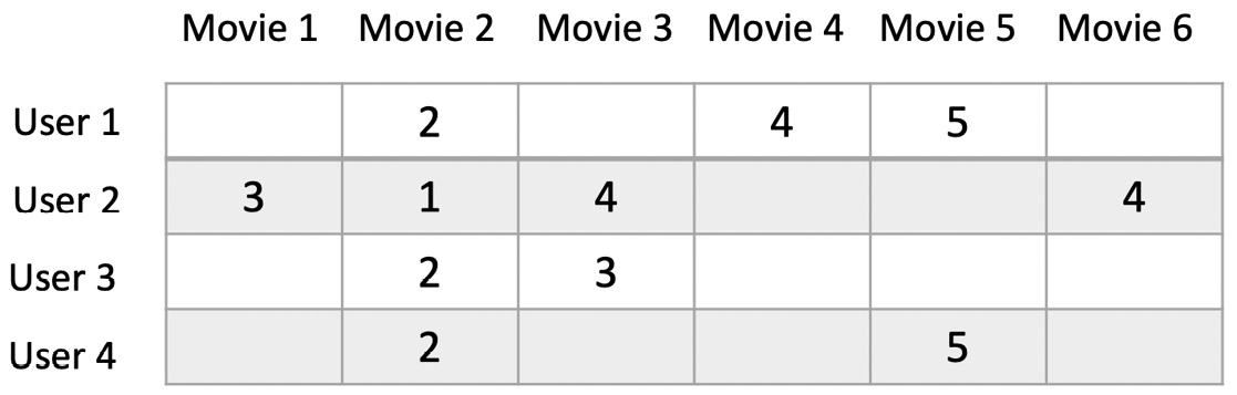
Figure 4.2 – Sparse matrix

Hence, the matrix would have 943*1,682=1,586,126 cells. However, as only 100,000 ratings are present, 93.69% of cells would be empty. Storing our dataset this way would be extremely inefficient. It would needlessly consume RAM, storage, and network bandwidth to store and transfer lots of zero values!

In fact, things are much worse, as the algorithm expects the input dataset to look like in the following diagram:

Figure 4.3 – Sparse matrix

Why do we need to store data this way? The answer is simple: Factorization Machines is a supervised learning algorithm, so we need to train it on labeled samples.

Looking at the preceding diagram, we see that each line represents a movie review. The matrix on the left stores its one-hot encoded features (users and movies), and the vector on the right stores its label. For instance, the last line tells us that user 4 has given movie 5 a "5" rating.

The size of this matrix is 100,000 lines by 2,625 columns (943 movies plus 1,682 movies). The total number of cells is 262,500,000, which are only 0.076% full (200,000 / 262,500,000). If we used a 32-bit value for each cell, we would need almost a gigabyte of memory to store this matrix. This is horribly inefficient, but still manageable.

Just for fun, let's do the same exercise for the largest version of MovieLens, which has 25 million ratings, 62,000 movies and 162,000 users. The matrix would have 25 million lines and 224,000 columns, for a total of 5,600,000,000,000 cells. Yes, that's 5.6 trillion cells, and although they would be 99.999% empty, we would still need over 20 terabytes of RAM to store them. Ouch. If that's not bad enough, consider recommendation models with millions of users and products: the numbers are mind-boggling!

Instead of using a plain matrix, we'll use a sparse matrix, a data structure specifically designed and optimized for sparse datasets. Scipy has exactly the object we need, named lil_matrix (https://docs.scipy.org/doc/scipy/reference/generated/scipy.sparse.lil_matrix.html). This will help us to get rid of all these nasty zeros.

Understanding protobuf and RecordIO

So how will we pass this sparse matrix to the SageMaker algorithm? As you would expect, we're going to serialize the object, and store it in S3. We're not going to use Python serialization, however. Instead, we're going to use protobuf (https://developers.google.com/protocol-buffers/), a popular and efficient serialization mechanism.

In addition, we're going to store the protobuf-encoded data in a record format called RecordIO (https://mxnet.apache.org/api/faq/recordio/). Our dataset will be stored as a sequence of records in a single file. This has the following benefits:

• A single file is easier to move around: who wants to deal with thousands of individual files that can get lost or corrupted?
• A sequential file is faster to read, which makes the training process more efficient.
• A sequence of records is easy to split for distributed training.

Don't worry if you're not familiar with protobuf and RecordIO. The SageMaker SDK includes utility functions that hide their complexity.

Building a Factorization Machines model on MovieLens

We will begin building the model using the following steps:

1. In a Jupyter notebook, we first download and extract the MovieLens dataset:

   %%sh wget http://files.grouplens.org/datasets/movielens/ml-100k.zip
unzip ml-100k.zip

2. As the dataset is ordered by user ID, we shuffle it as a precaution. Then, we take a look at the first few lines:

   %cd ml-100k !shuf ua.base -o ua.base.shuffled !head -5 ua.base.shuffled

   We see four columns: the user ID, the movie ID, the rating, and a timestamp (which we'll ignore in our model):

   378 43 3 880056609 919 558 5 875372988 90 285 5 891383687 249 245 2 879571999 416 64 5 893212929

3. We define sizing constants:

   num_users = 943 num_movies = 1682 num_features = num_users+num_movies

   num_ratings_train = 90570 num_ratings_test = 9430

4. Now, let's write a function to load a dataset into a sparse matrix. Based on the previous explanation, we go through the dataset line by line. In the X matrix, we set the appropriate user and movie columns to 1. We also store the rating in the Y vector:

   import csv import numpy as np from scipy.sparse import lil_matrix

   def loadDataset(filename, lines, columns):

       X = lil_matrix((lines, columns)).astype('float32')    Y = []

       line=0     with open(filename,'r') as f:        samples=csv.reader(f,delimiter=' ')        for userId,movieId,rating,timestamp in samples:            X[line,int(userId)-1] = 1             X[line,int(num_users)+int(movieId)-1] = 1             Y.append(int(rating))            line=line+1           Y=np.array(Y).astype('float32')    return X,Y

5. We then process the training and test datasets:

   X_train, Y_train = loadDataset('ua.base.shuffled',                                num_ratings_train,                                 num_features)

   X_test, Y_test = loadDataset('ua.test',                             num_ratings_test,                              num_features)

6. We check that the shapes are what we expect:

   print(X_train.shape)print(Y_train.shape)print(X_test.shape)print(Y_test.shape)

   This displays the dataset shapes:

   (90570, 2625)(90570,)(9430, 2625)(9430,)

7. Now, let's write a function that converts a dataset to the RecordIO-wrapped protobuf, and uploads it to an S3 bucket. We first create an in-memory binary stream with io.BytesIO(). Then, we use the life-saving write_spmatrix_to_sparse_tensor() function to write the sample matrix and the label vector to that buffer in protobuf format. Finally, we use boto3 to upload the buffer to S3:

   import io, boto3 import sagemaker.amazon.common as smac

   def writeDatasetToProtobuf(X, Y, bucket, prefix, key):    buf = io.BytesIO()    smac.write_spmatrix_to_sparse_tensor(buf, X, Y)    buf.seek(0)    obj = '{}/{}'.format(prefix, key)          boto3.resource('s3').Bucket(bucket).Object(obj).    upload_fileobj(buf)

       return 's3://{}/{}'.format(bucket,obj)

   Had our data been stored in a numpy array instead of lilmatrix, we would have used the write_numpy_to_dense_tensor() function instead. It has the same effect.

8. We apply this function to both datasets, and we store their S3 paths:

   import sagemaker

   bucket = sagemaker.Session().default_bucket()prefix = 'fm-movielens'

   train_key      = 'train.protobuf'train_prefix   = '{}/{}'.format(prefix, 'train')

   test_key       = 'test.protobuf'test_prefix    = '{}/{}'.format(prefix, 'test')

   output_prefix  = 's3://{}/{}/output'.format(bucket,                                             prefix)

   train_data = writeDatasetToProtobuf(X_train, Y_train,              bucket, train_prefix, train_key)    

   test_data  = writeDatasetToProtobuf(X_test, Y_test,              bucket, test_prefix, test_key)    

9. Taking a look at the S3 bucket in a terminal, we see that the training dataset only takes 5.5 MB. The combination of sparse matrix, protobuf, and RecordIO has paid off:

   $ aws s3 ls s3://sagemaker-eu-west-1-123456789012/fm-movielens/train/train.protobuf

   5796480 train.protobuf

10. What comes next is SageMaker business as usual. We find the name of the Factorization Machines container, configure the Estimator function, and set the hyperparameters:

    from sagemaker import image_uris

    region=boto3.Session().region_name

    container=image_uris.retrieve('factorization-machines', region)

    fm=sagemaker.estimator.Estimator(    container,    role=sagemaker.get_execution_role(),    instance_count=1,    instance_type='ml.c5.xlarge',    output_path=output_prefix)

    fm.set_hyperparameters(    feature_dim=num_features,    predictor_type='regressor',    num_factors=64,    epochs=10)

    Looking at the documentation (https://docs.aws.amazon.com/sagemaker/latest/dg/fact-machines-hyperparameters.html), we see that the required hyperparameters are feature_dim, predictor_type, and num_factors. The default setting for epochs is 1, which feels a little low, so we use 10 instead.

11. We then launch the training job. Did you notice that we didn't configure training inputs? We're simply passing the location of the two protobuf files. As protobuf is the default format for Factorization Machines (as well as other built-in algorithms), we can save a step:

    fm.fit({'train': train_data, 'test': test_data})

12. Once the job is over, we deploy the model to a real-time endpoint:

    endpoint_name = 'fm-movielens-100k'

    fm_predictor = fm.deploy(    endpoint_name=endpoint_name,    instance_type='ml.t2.medium',     initial_instance_count=1)

13. We'll now send samples to the endpoint in JSON format (https://docs.aws.amazon.com/sagemaker/latest/dg/fact-machines.html#fm-inputoutput). For this purpose, we write a custom serializer to convert input data to JSON. The default JSON deserializer will be used automatically since we set the content type to 'application/json':

    import json

    def fm_serializer(data):    js = {'instances': []}    for row in data:        js['instances'].append({'features':                                 row.tolist()})    return json.dumps(js)

    fm_predictor.content_type = 'application/json'fm_predictor.serializer = fm_serializer

14. We send the first three samples of the test set for prediction:

    result = fm_predictor.predict(X_test[:3].toarray())print(result)

    The prediction looks like this:

    {'predictions': [{'score': 3.3772034645080566}, {'score': 3.4299235343933105}, {'score': 3.6053106784820557}]}

15. Using this model, we could fill all the empty cells in the recommendation matrix. For each user, we would simply predict the score of all movies, and store say the top 50 movies. That information would be stored in a backend, and the corresponding metadata (title, genre, and so on) would be displayed to the user in a frontend application.
16. Finally, we delete the endpoint:

    fm_predictor.delete_endpoint()

So far, we've only used supervised learning algorithms. In the next section, we'll move on to unsupervised learning with Principal Component Analysis.

Using Principal Component Analysis

Principal Component Analysis (PCA) is a dimension reductionality algorithm. It's often applied as a preliminary step before regression or classification. Let's use it on the protobuf dataset built in the Factorization Machines example. Its 2,625 columns are a good candidate for dimensionality reduction! We will use PCA by observing the following steps:

1. Starting from the processed dataset, we configure the Estimator for PCA. By now, you should (almost) be able to do this with your eyes closed:

   import boto3 from sagemaker import image_uris

   region = boto3.Session().region_name    container = image_uris.retrieve('pca', region)

   pca = sagemaker.estimator.Estimator(    container=container,    role=sagemaker.get_execution_role(),    instance_count=1,                                   instance_type='ml.c5.xlarge',
    output_path=output_prefix)

2. We then set the hyperparameters. The required ones are the initial number of features, the number of principal components to compute, and the batch size:

   pca.set_hyperparameters(feature_dim=num_features,                        num_components=64,                        mini_batch_size=1024)

3. We train and deploy the model:

   pca.fit({'train': train_data, 'test': test_data})pca_predictor = pca.deploy(    endpoint_name='pca-movielens-100k',    instance_type='ml.t2.medium',    initial_instance_count=1)

4. Then, we predict the first test sample, using the same serialization code as in the previous example:

   import json

   def pca_serializer(data):    js = {'instances': []}    for row in data:        js['instances'].append({'features':                                 row.tolist()})    return json.dumps(js)

   pca_predictor.content_type = 'application/json'pca_predictor.serializer = pca_serializer

   result = pca_predictor.predict(X_test[0].toarray())

   print(result)

   This prints out the 64 principal components of the test sample. In real life, we typically would process the dataset with this model, save the results, and use them to train a regression model:

   {'projections': [{'projection': [-0.008711372502148151, 0.0019895541481673717, 0.002355781616643071, 0.012406938709318638, -0.0069608548656105995, -0.009556426666676998, <output removed>]}]}

Don't forget to delete the endpoint when you're done. Then, let's run one more unsupervised learning example to conclude this chapter!

Detecting anomalies with Random Cut Forest

Random Cut Forest (RCF) is an unsupervised learning algorithm for anomaly detection (https://proceedings.mlr.press/v48/guha16.pdf). We're going to apply it to a subset of the household electric power consumption dataset (https://archive.ics.uci.edu/ml/), available in the GitHub repository for this book. The data has been aggregated hourly over a period of little less than a year (just under 8,000 values):

1. In a Jupyter notebook, we load the dataset with pandas, and we display the first few lines:

   import pandas as pd

   df = pd.read_csv('item-demand-time.csv', dtype = object, names=['timestamp','value','client'])

   df.head(3)

   As shown in the following screenshot, the dataset has three columns: an hourly timestamp, the power consumption value (in kilowatt-hours), and the client ID:

   

   Figure 4.4 – Viewing the columns

2. Using matplotlib, we plot the dataset to get a quick idea of what it looks like:

   import matplotlib import matplotlib.pyplot as plt

   df.value=pd.to_numeric(df.value)df_plot=df.pivot(index='timestamp',columns='item',                 values='value')df_plot.plot(figsize=(40,10))

   The plot is shown in the following diagram. We see three time series corresponding to three different clients:

   

   Figure 4.5 – Viewing the dataset

3. There are two issues with this dataset. First, it contains several time series: RCF can only train a model on a single series. Second, RCF requires integer values. Let's solve both problem with pandas: we only keep the "client_12" time series, we multiply its values by 100, and cast them to the integer type:

   df = df[df['item']=='client_12']df = df.drop(['item', 'timestamp'], axis=1)df.value *= 100 df.value = df.value.astype('int32')df.head()

   The following diagram shows the first lines of the transformed dataset:

   

   Figure 4.6 – The values of the first lines

4. We plot it again to check that it looks like expected. Note the large drop right after step 2,000, highlighted by a box in the following diagram. This is clearly an anomaly, and hopefully our model will catch it:
   

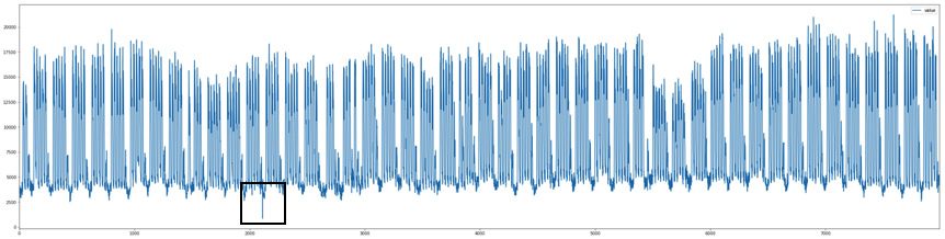
   Figure 4.7 – Viewing a single time series

5. As in the previous examples, we save the dataset to a CSV file, which we upload to S3:

   import boto3 import sagemaker

   sess = sagemaker.Session()bucket = sess.default_bucket()prefix = 'electricity'

   df.to_csv('electricity.csv', index=False, header=False)

   training_data_path = sess.upload_data(                       path='electricity.csv',                        key_prefix=prefix +                                   '/input/training')

6. Then, we define the training channel. There are a couple of quirks that we haven't met before. SageMaker generally doesn't have many of these, and reading the documentation goes a long way in pinpointing them (https://docs.aws.amazon.com/sagemaker/latest/dg/randomcutforest.html).

   First, the content type must state that data is not labeled. The reason for this is that RCF can accept an optional test channel where anomalies are labeled (label_size=1). Even though the training channel never has labels, we still need to tell RCF. Second, the only distribution policy supported in RCF is ShardedByS3Key. This policy splits the dataset across the different instances in the training cluster, instead of sending them a full copy. We won't run distributed training here, but we need to set that policy nonetheless:

   training_data_channel =     sagemaker.TrainingInput(        s3_data=training_data_path,        content_type='text/csv;label_size=0',        distribution='ShardedByS3Key')

   rcf_data = {'train': training_data_channel}

7. The rest is business as usual: train and deploy! Once again, we reuse the code for the previous examples, and it's almost unchanged:

   from sagemaker.estimator import Estimator from sagemaker import image_uris

   role = sagemaker.get_execution_role()region = boto3.Session().region_name container = image_uris.retrieve('randomcutforest',                                 region)

   rcf_estimator = Estimator(container,    role=role,    instance_count=1,    instance_type='ml.m5.large',    output_path='s3://{}/{}/output'.format(bucket,                                            prefix))

   rcf_estimator.set_hyperparameters(feature_dim=1)rcf_estimator.fit(rcf_data)

   endpoint_name = 'rcf-demo'rcf_predictor = rcf_estimator.deploy(    endpoint_name=endpoint_name,    initial_instance_count=1,    instance_type='ml.t2.medium')

8. After a few minutes, the model is deployed. We convert the input time series to a Python list, and we send it to the endpoint for prediction. We use CSV and JSON, respectively, for serialization and deserialization:

   rcf_predictor.content_type = 'text/csv'rcf_predictor.serializer =    sagemaker.serializers.CSVSerializer()

   rcf_predictor.deserializer =    sagemaker.deserializers.JSONDeserializer()

   values = df['value'].astype('str').tolist()response = rcf_predictor.predict(values)print(response)

   The response contains the anomaly score for each value in the time series. It looks like this:

   {'scores': [{'score': 1.0868037776}, {'score': 1.5307718138}, {'score': 1.4208102841} …

9. We then convert this response to a Python list, and we then compute its mean and its standard deviation:

   from statistics import mean,stdev

   scores = []for s in response['scores']:    scores.append(s['score'])

   score_mean = mean(scores)score_std = stdev(scores)

10. We plot a subset of the time series and the corresponding scores. Let's focus on the [2000-2500] interval, as this is where we saw a large drop. We also plot a line representing the mean plus three standard deviations (99.7% of the score distribution): any score largely exceeding the line is likely to be an anomaly:

    df[2000:2500].plot(figsize=(40,10))

    plt.figure(figsize=(40,10))plt.plot(scores[2000:2500])plt.autoscale(tight=True)plt.axhline(y=score_mean+3*score_std, color='red')plt.show()

    The drop is clearly visible in the following plot:

    

    Figure 4.8 – Zooming in on an anomaly

    As you can see on the following score plot, its score is sky high! Beyond a doubt, this value is an anomaly:

    

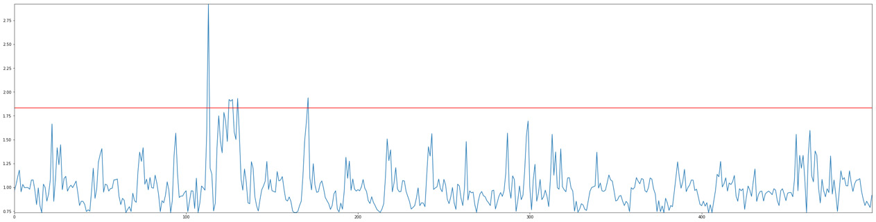
    Figure 4.9 – Viewing anomaly scores

    Exploring other intervals of the time series, we could certainly find more. Who said machine learning wasn't fun?

11. Finally, we delete the endpoint:

    rcf_predictor.delete_endpoint()

Having gone through five complete examples, you should now be familiar with built-in algorithms, the SageMaker workflow, and the SDK. To fully master these topics, I would recommend experimenting with your datasets, and running the additional examples available at https://github.com/awslabs/amazon-sagemaker-examples/tree/master/introduction_to_amazon_algorithms.

Summary

As you can see, built-in algorithms are a great way to quickly train and deploy models without having to write any machine learning code.

In this chapter, you learned about the SageMaker workflow, and how to implement it with a handful of APIs from the SageMaker SDK, without ever worrying about infrastructure.

You learned how to work with data in CSV and RecordIO-wrapped protobuf format, the latter being the preferred format for large-scale training on bulky datasets.You also learned how to build models with important algorithms for supervised and unsupervised learning: Linear Learner, XGBoost, Factorization Machines, PCA, and Random Cut Forest.

In the next chapter, you will learn how to use additional built-in algorithms to build computer vision models.