Chapter 2: Handling Data Preparation Techniques

Data is the starting point of any machine learning project, and it takes lots of work to turn data into a dataset that can be used to train a model. That work typically involves annotating datasets, running bespoke scripts to preprocess them, and saving processed versions for later use. As you can guess, doing all this work manually, or building tools to automate it, is not an exciting prospect for machine learning teams.

In this chapter, you will learn about AWS services that help you build and process data. We'll first cover Amazon SageMaker Ground Truth, a capability of Amazon SageMaker that helps you quickly build accurate training datasets. Then, we'll talk about Amazon SageMaker Processing, another capability that helps you run your data processing workloads, such as feature engineering, data validation, model evaluation, and model interpretation. Finally, we'll discuss other AWS services that may help with data analytics: Amazon Elastic Map Reduce, AWS Glue, and Amazon Athena:

• Discovering Amazon SageMaker Ground Truth
• Exploring Amazon SageMaker Processing
• Processing data with other AWS services

Technical requirements

You will need an AWS account to run examples included in this chapter. If you haven't got one already, please point your browser at https://aws.amazon.com/getting-started/ to create one. You should also familiarize yourself with the AWS Free Tier (https://aws.amazon.com/free/), which lets you use many AWS services for free within certain usage limits.

You will need to install and to configure the AWS Command-Line Interface (CLI) for your account (https://aws.amazon.com/cli/).

You will need a working Python 3.x environment. Be careful not to use Python 2.7, as it is no longer maintained. Installing the Anaconda distribution (https://www.anaconda.com/) is not mandatory, but strongly encouraged as it includes many projects that we will need (Jupyter, pandas, numpy, and more).

Code examples included in the book are available on GitHub at https://github.com/PacktPublishing/Learn-Amazon-SageMaker. You will need to install a Git client to access them (https://git-scm.com/).

Discovering Amazon SageMaker Ground Truth

Added to Amazon SageMaker in late 2018, Amazon SageMaker Ground Truth helps you quickly build accurate training datasets. Machine learning practitioners can distribute labeling work to public and private workforces of human labelers. Labelers can be productive immediately, thanks to built-in workflows and graphical interfaces for common image, video, and text tasks. In addition, Ground Truth can enable automatic labeling, a technique that trains a machine learning model able to label data without additional human intervention.

In this section, you'll learn how to use Ground Truth to label images and text.

Using workforces

The first step in using Ground Truth is to create a workforce, a group of workers in charge of labeling data samples.

Let's head out to the SageMaker console: in the left-hand vertical menu, we click on Ground Truth, then on Labeling workforces. Three types of workforces are available: Amazon Mechanical Turk, Vendor, and Private. Let's discuss what they are, and when you should use them.

Amazon Mechanical Turk

Amazon Mechanical Turk (https://www.mturk.com/) makes it easy to break down large batch jobs into small work units that can be processed by a distributed workforce.

With Mechanical Turk, you can enroll tens or even hundreds of thousands of workers located across the globe. This is a great option when you need to label extremely large datasets. For example, think about a dataset for autonomous driving, made up of 1000 hours of video: each frame would need to be processed in order to identify other vehicles, pedestrians, road signs, and more. If you wanted to annotate every single frame, you'd be looking at 1,000 hours x 3,600 seconds x 24 frames per second = 86.4 million images! Clearly, you would have to scale out your labeling workforce to get the job done, and Mechanical Turk lets you do that.

Vendor workforce

As scalable as Mechanical Turk is, sometimes you need more control on who data is shared with, and on the quality of annotations, particularly if additional domain knowledge is required.

For this purpose, AWS has vetted a number of data labeling companies, which have integrated Ground Truth in their workflows. You can find the list of companies on AWS Marketplace (https://aws.amazon.com/marketplace/), under Machine Learning | Data Labeling Services | Amazon SageMaker Ground Truth Services.

­Private workforce

Sometimes, data can't be processed by third parties. Maybe it's just too sensitive, or maybe it requires expert knowledge that only your company's employees have. In this case, you can create a private workforce, made up of well-identified individuals that will access and label your data.

Creating a private workforce

Creating a private workforce is the quickest and simplest option. Let's see how it's done:

1. Starting from the Labeling workforces entry in the SageMaker console, we select the Private tab, as seen in the following screenshot. Then, we click on Create private team:
   

   Figure 2.1 – Creating a private workforce

2. We give the team a name, then we have to decide whether we're going to invite workers by email, or whether we're going to import users that belong to an existing Amazon Cognito group.

   Amazon Cognito (https://aws.amazon.com/cognito/) is a managed service that lets you build and manage user directories at any scale. Cognito supports both social identity providers (Google, Facebook, and Amazon), and enterprise identity providers (Microsoft Active Directory, SAML).

   This makes a lot of sense in an enterprise context, but let's keep things simple and use email instead. Here, I will use some sample email addresses: please make sure to use your own, otherwise you won't be able to join the team!

3. Then, we need to enter an organization name, and more importantly a contact email that workers can use for questions and feedback on the labeling job. These conversations are extremely important in order to fine-tune labeling instructions, pinpoint problematic data samples, and more.
4. Optionally, we can set up notifications with Amazon Simple Notification Service (https://aws.amazon.com/sns/), to let workers know that they have work to do.
5. The screen should look like in the following screenshot. Then, we click on Create private team:
   

   ­

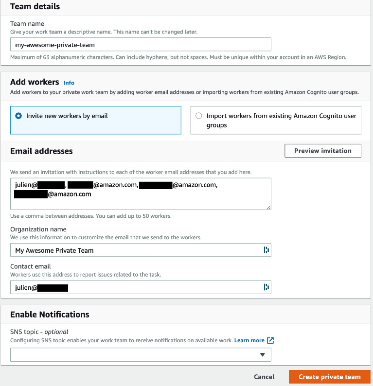
   Figure 2.2 – Setting up a private workforce

6. A few seconds later, the team has been set up. Invitations have been sent to workers, requesting that they join the workforce by logging in to a specific URL. The invitation email looks like that shown in the following screenshot:
   

   Figure 2.3 – Email invitation

7. Clicking on the link opens a login window. Once we've logged in and defined a new password, we're taken to a new screen showing available jobs, as in the following screenshot. As we haven't defined one yet, it's obviously empty:

Figure 2.4 – Worker console

Let's keep our workers busy and create an image labeling job.

Uploading data for labeling

As you would expect, Amazon SageMaker Ground Truth uses Amazon S3 to store datasets:

1. Using the AWS CLI, we create an S3 bucket hosted in the same region we're running SageMaker in. Bucket names are globally unique, so please make sure to pick your own unique name when you create the bucket. Use the following code:

   $ aws s3 mb s3://sagemaker-book --region eu-west-1

2. Then, we copy the cat images located in the chapter2 folder of our GitHub repository as follows:

   $ aws s3 cp --recursive cat/ s3://sagemaker-book/chapter2/cat/

Now that we have some data waiting to be labeled, let's create a labeling job.

Creating a labeling job

As you would expect, we need to define the location of the data, what type of task we want to label it for, and what our instructions are:

1. In the left-hand vertical menu of the SageMaker console, we click on Ground Truth, then on Labeling jobs, then on the Create labeling job button.
2. First, we give the job a name, say my-cat-job. Then, we define the location of the data in S3. Ground Truth expects a manifest file: a manifest file is a JSON file that lets you filter which objects need to be labeled, and which ones should be left out. Once the job is complete, a new file, called the augmented manifest, will contain labeling information, and we'll be able to use this to feed data to training jobs.
3. Then, we define the location and the type of our input data, just like in the following screenshot:
   

   Figure 2.5 – Configuring input data

4. As is visible in the next screenshot, we select the IAM role that we created for SageMaker in the first chapter (your name will be different), and we then click on the Complete data setup button to validate this section:
   

   Figure 2.6 – Validating input data

   Clicking on View more details, you can learn about what is happening under the hood. SageMaker Ground Truth crawls your data in S3 and creates a JSON file called the manifest file. You can go and download it from S3 if you're curious. This file points at your objects in S3 (images, text files, and so on).

5. Optionally, we could decide to work either with the full manifest, a random sample, or a filtered subset based on a SQL query. We could also provide an Amazon KMS key to encrypt the output of the job. Let's stick to the defaults here.
6. The Task type section asks us what kind of job we'd like to run. Please take a minute to explore the different task categories that are available (text, image, video, point cloud, and custom). You'll see that SageMaker Ground Truth can help you with the following tasks:

   a) Text classification

   b) Named entity recognition

   c) Image classification: Categorizing images in specific classes

   d) Object detection: Locating and labeling objects in images with bounding boxes

   e) Semantic segmentation: Locating and labeling objects in images with pixel-level precision

   f) Video clip classification: Categorizing videos in specific classes

   g) Multi-frame video object detection and tracking

   h) 3D point clouds: Locating and labeling objects in 3D data, such as LIDAR data for autonomous driving

   i) Custom user-defined tasks

   As shown in the next screenshot, let's select the Image task category and the Semantic segmentation task, and then click Next:

   

   Figure 2.7 – Selecting a task type

7. On the next screen, visible in the following screenshot, we first select our private team of workers:
   

   Figure 2.8 – Selecting a team type

8. If we had a lot of samples (say, tens of thousands or more), we should consider enabling automated data labeling, as this feature would reduce both the duration and the cost of the labeling job. Indeed, as workers would start labeling data samples, SageMaker Ground Truth would train a machine learning model on these samples. It would use them as a dataset for a supervised learning problem. With enough worker-labeled data, this model would pretty quickly be able to match and exceed human accuracy, at which point it would replace workers and label the rest of the dataset. If you'd like to know more about this feature, please read the documentation at https://docs.aws.amazon.com/sagemaker/latest/dg/sms-automated-labeling.html.
9. The last step in configuring our training job is to enter instructions for the workers. This is an important step, especially if your job is distributed to third-party workers. The better our instructions, the higher the quality of the annotations. Here, let's explain what the job is about, and enter a cat label for workers to apply. In a real-life scenario, you should add detailed instructions, provide sample images for good and bad examples, explain what your expectations are, and so on. The following screenshot shows what our instructions look like:
   

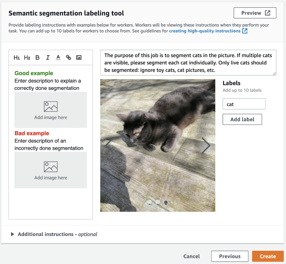
   Figure 2.9 – Setting up instructions

10. Once we're done with instructions, we click on Create to launch the labeling job. After a few minutes, the job is ready to be distributed to workers.

Labeling images

Logging in to the worker URL, we can see from the screen shown in the following screenshot that we have work to do:

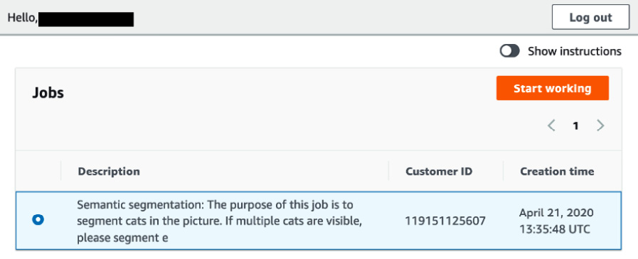
Figure 2.10 – Worker console

1. Clicking on Start working opens a new window, visible in the next picture. It displays instructions as well as a first image to work on:
   

   Figure 2.11 – Labeling images

2. Using the graphical tools in the toolbar, and especially the auto-segment tool, we can very quickly produce high-quality annotations. Please take a few minutes to practice, and you'll be able to do the same in no time.
3. Once we're done with the three images, the job is complete, and we can visualize the labeled images under Labeling jobs in the SageMaker console. Your screen should look like the following screenshot:

Figure 2.12 – Labeled images

More importantly, we can find labeling information in the S3 output location.

In particular, the augmented manifest (output/my-cat-job/manifests/output/output.manifest) contains annotation information on each data sample, such as the classes present in the image, and a link to the segmentation mask:

{"source-ref":"s3://sagemaker-book/chapter2/cat/cat1.jpg","my-cat-job-ref":"s3://sagemaker-book/chapter2/cat/output/my-cat-job/annotations/consolidated-annotation/output/0_2020-04-21T13:48:00.091190.png","my-cat-job-ref-metadata":{"internal-color-map":{"0":{"class-name":"BACKGROUND","hex-color":"#ffffff","confidence":0.8054600000000001},"1":{"class-name":"cat","hex-color":"#2ca02c","confidence":0.8054600000000001}},"type":"groundtruth/semantic-segmentation","human-annotated":"yes","creation-date":"2020-04-21T13:48:00.562419","job-name":"labeling-job/my-cat-job"}}

Yes, that's quite a mouthful! Don't worry though: in Chapter 5, Training Computer Vision Models, we'll see how we can feed this information directly to the built-in computer vision algorithms implemented in Amazon SageMaker. Of course, we could also parse this information, and convert it for whatever framework we use to train our computer vision model.

As you can see, SageMaker Ground Truth makes it easy to label image datasets. You just need to upload your data to S3 and create a workforce. Ground Truth will then distribute the work automatically, and store the results in S3.

We just saw how to label images, but what about text tasks? Well, they're equally easy to set up and run. Let's go through an example.

Labeling text

This is a quick example of labeling text for named entity recognition. The dataset is made up of text fragments from one of my blog posts, where we'd like to label all AWS service names. These are available in our GitHub repository:

$ cat ner/1.txt With great power come great responsibility. The second you create AWS resources, you're responsible for them: security of course, but also cost and scaling. This makes monitoring and alerting all the more important, which is why we built services like Amazon CloudWatch, AWS Config and AWS Systems Manager.

We will start labeling text using the following steps:

1. First, let's upload text fragments to S3 with the following line of code:

   $ aws s3 cp --recursive ner/ s3://sagemaker-book/chapter2/ner/

2. Just like in the previous example, we configure a text labeling job, set up input data, and select an IAM role, as shown in the following screenshot:
   

   Figure 2.13 – Creating a text labeling job

3. Then, we select Text as the category, and Named entity recognition as the task.
4. On the next screen, shown in the following screenshot, we simply select our private team again, add a label, and enter instructions:
   

   Figure 2.14 – Setting up instructions

5. Once the job is ready, we log in to the worker console and start labeling. You can see a labeled example in the following screenshot:
   

   Figure 2.15 – Labeling text

6. We're done quickly, and we can find the labeling information in our S3 bucket. Here's what we find for the preceding text: for each entity, we get a start offset, an end offset, and a label:

   {"source": "Since 2006, Amazon Web Services has been striving to simplify IT infrastructure. Thanks to services like Amazon Elastic Compute Cloud (EC2),Amazon Simple Storage Service (S3), Amazon Relational Database Service (RDS), AWS CloudFormation and many more,millions of customers can build reliable, scalable, and secure platforms in any AWS region in minutes. Having spent 10 years procuring, deploying and managing more hardware than I care to remember, I'm still amazed every day by the pace of innovation that builders achieve with our services.","my-ner-job": {"annotations": {"entities":[{"endOffset":133,"startOffset":105,"label":"aws_service"}, {"endOffset":138,"startOffset":135,"label":"aws_service"},{"endOffset":170,"startOffset":141,"label":"aws_service"}, {"endOffset":174,"startOffset":172,"label":"aws_service"}, {"endOffset":211,"startOffset":177,"label":"aws_service"}, {"endOffset":216,"startOffset":213,"label":"aws_service"}, {"endOffset":237,"startOffset":219,"label":"aws_service"}], "labels":[{"label":"aws_service"}]}}, "my-ner-job-metadata": {"entities":[{"confidence":0.12},{"confidence":0.08},{"confidence":0.13},{"confidence":0.07},{"confidence":0.14},{"confidence":0.08},{"confidence":0.1}],"job-name":"labeling-job/my-ner-job","type":"groundtruth/text-span","creation-date":"2020-04-21T14:32:36.573013","human-annotated":"yes"}}

Amazon SageMaker Ground Truth really makes it easy to label datasets at scale. It has many nice features including job chaining and custom workflows, which I encourage you to explore at https://docs.aws.amazon.com/sagemaker/latest/dg/sms.html.

Next, we're going to learn about Amazon SageMaker Processing, and you can easily use it to process any dataset using your own code.

Exploring Amazon SageMaker Processing

Collecting and labeling data samples is only the first step in preparing a dataset. Indeed, it's very likely that you'll have to pre-process your dataset in order to do the following, for example:

• Convert it to the input format expected by the machine learning algorithm you're using.
• Rescale or normalize numerical features.
• Engineer higher-level features, for example, one-hot encoding.
• Clean and tokenize text for natural language processing applications.
• And more!

Once training is complete, you may want to run additional jobs to post-process the predicted data and to evaluate your model on different datasets.

In this section, you'll learn about Amazon SageMaker Processing, a SageMaker capability that helps you run batch jobs related to your machine learning project.

Discovering the Amazon SageMaker Processing API

The Amazon SageMaker Processing API is part of the SageMaker SDK, which we already installed in Chapter 1, Introducing Amazon SageMaker. Its documentation is available at https://sagemaker.readthedocs.io.

SageMaker Processing provides you with a built-in Docker container that can run Python batch jobs written with scikit-learn (https://scikit-learn.org). You can also use your own container if you'd like. Logs are available in Amazon CloudWatch Logs in the /aws/sagemaker/ProcessingJobs log group.

Let's first see how we can use scikit-learn and SageMaker Processing to prepare a dataset for training.

Note:

You can run this example, and all future examples, either on your local machine, on a Notebook instance, or in SageMaker Studio. Please make sure to enable the appropriate conda or virtualenv environment, as explained in Chapter 1, Getting Started with Amazon SageMaker .

For the rest of the book, I also recommend that you follow along and run the code available in the companion GitHub repository. Every effort has been made to check all code samples present in the text. However, for those of you who have an electronic version, copying and pasting may have unpredictable results: formatting issues, weird quotes, and so on.

Processing a dataset with scikit-learn

Here's the high-level process:

• Upload your unprocessed dataset to Amazon S3.
• Write a script with scikit-learn in order to load the dataset, process it, and save the processed features and labels.
• Run this script with SageMaker Processing on managed infrastructure.

Uploading the dataset to Amazon S3

First, we need a dataset. We'll use the direct marketing dataset published by S. Moro, P. Cortez, and P. Rita in "A Data-Driven Approach to Predict the Success of Bank Telemarketing", Decision Support Systems, Elsevier, 62:22-31, June 2014.

This dataset describes a binary classification problem: will a customer accept a marketing offer, yes or no? It contains a little more than 41,000 labeled customer samples. Let's dive in:

1. Creating a new Jupyter notebook, let's first download and extract the dataset:

   %%sh

   apt-get -y install unzip    # Only needed in SageMaker Studio

   wget -N https://sagemaker-sample-data-us-west-2.s3-us-west-2.amazonaws.com/autopilot/direct_marketing/bank-additional.zip

   unzip -o bank-additional.zip

2. Then, we load it with pandas:

   import pandas as pd

   data = pd.read_csv('./bank-additional/bank-additional-full.csv')

   print(data.shape)(41188, 21)

3. ­­Now, let's display the first five lines:

   data[:5]

   This prints out the table visible in the following figure:

   

   Figure 2.16 – Viewing the dataset

   Scrolling to the right, we can see a column named y, storing the labels.

4. Now, let's upload the dataset to Amazon S3. We'll use a default bucket automatically created by SageMaker in the region we're running in. We'll just add a prefix to keep things nice and tidy:

   import sagemaker

   prefix = 'sagemaker/DEMO-smprocessing/input'

   input_data = sagemaker.Session().upload_data(path='./bank-additional/bank-additional-full.csv', key_prefix=prefix)

Writing a processing script with scikit-learn

As SageMaker Processing takes care of all infrastructure concerns, we can focus on the script itself. We don't have to worry about Amazon S3 either: SageMaker Processing will automatically copy the input dataset from S3 into the container, and the processed datasets from the container to S3.

Container paths are provided when we configure the job itself. Here's what we'll use:

• The input dataset: /opt/ml/processing/input
• The processed training set: /opt/ml/processing/train
• The processed test set: /opt/ml/processing/test

In our Jupyter environment, let's start writing a new Python file named preprocessing.py. As you would expect, this script will load the dataset, perform basic feature engineering, and save the processed dataset:

1. First, we read our single command-line parameter with the argparse library (https://docs.python.org/3/library/argparse.html): the ratio for the training and test datasets. The actual value will be passed to the script by the SageMaker Processing SDK:

   import argparse

   parser = argparse.ArgumentParser()parser.add_argument('--train-test-split-ratio',                     type=float, default=0.3)args, _ = parser.parse_known_args()print('Received arguments {}'.format(args))split_ratio = args.train_test_split_ratio

2. We load the input dataset using pandas. At startup, SageMaker Processing automatically copied it from S3 to a user-defined location inside the container; here, it is /opt/ml/processing/input:

   import os import pandas as pd

   input_data_path = os.path.join('/opt/ml/processing/input', 'bank-additional-full.csv')

   df = pd.read_csv(input_data_path)

3. Then, we remove any line with missing values, as well as duplicate lines:

   df.dropna(inplace=True)df.drop_duplicates(inplace=True)

4. Then, we count negative and positive samples, and display the class ratio. This will tell us how unbalanced the dataset is:

   one_class = df[df['y']=='yes']one_class_count = one_class.shape[0]zero_class = df[df['y']=='no']zero_class_count = zero_class.shape[0]zero_to_one_ratio = zero_class_count/one_class_count print("Ratio: %.2f" % zero_to_one_ratio)    

5. Looking at the dataset, we can see a column named pdays, telling us how long ago a customer has been contacted. Some lines have a 999 value, and that looks pretty suspicious: indeed, this is a placeholder value meaning that a customer has never been contacted. To help the model understand this assumption, let's add a new column stating it explicitly:

   import numpy as np

   df['no_previous_contact'] = np.where(df['pdays'] == 999, 1, 0)

6. In the job column, we can see three categories (student, retired, and unemployed) that should probably be grouped to indicate that these customers don't have a full-time job. Let's add another column:

   df['not_working'] = np.where(np.in1d(df['job'], ['student', 'retired', 'unemployed']), 1, 0)

7. Now, let's split the dataset into training and test sets. Scikit-learn has a convenient API for this, and we set the split ratio according to a command-line argument passed to the script:

   from sklearn.model_selection import train_test_split

   X_train, X_test, y_train, y_test = train_test_split(        df.drop('y', axis=1),        df['y'],        test_size=split_ratio, random_state=0)

8. The next step is to scale numerical features and to one-hot encode the categorical features. We'll use StandardScaler for the former, and OneHotEncoder for the latter:

   from sklearn.compose import make_column_transformer from sklearn.preprocessing import StandardScaler,OneHotEncoder

   preprocess = make_column_transformer(  (['age', 'duration', 'campaign', 'pdays', 'previous'],  StandardScaler()),  (['job', 'marital', 'education', 'default', 'housing',     'loan','contact', 'month', 'day_of_week',     'poutcome'],      OneHotEncoder(sparse=False)))

9. Then, we process the training and test datasets:

   train_features = preprocess.fit_transform(X_train)

   test_features = preprocess.transform(X_test)

10. Finally, we save the processed datasets, separating the features and labels. They're saved to user-defined locations in the container, and SageMaker Processing will automatically copy the files to S3 before terminating the job:

    train_features_output_path = os.path.join('/opt/ml/processing/train', 'train_features.csv')train_labels_output_path = os.path.join('/opt/ml/processing/train', 'train_labels.csv')

    test_features_output_path = os.path.join('/opt/ml/processing/test', 'test_features.csv')test_labels_output_path = os.path.join('/opt/ml/processing/test', 'test_labels.csv')

    pd.DataFrame(train_features).to_csv(train_features_output_path, header=False, index=False)pd.DataFrame(test_features).to_csv(test_features_output_path, header=False, index=False)

    y_train.to_csv(train_labels_output_path, header=False, index=False)y_test.to_csv(test_labels_output_path, header=False, index=False)

That's it. As you can see, this code is vanilla scikit-learn, so it shouldn't be difficult to adapt your own scripts for SageMaker Processing. Now let's see how we can actually run this.

Running a processing script

Coming back to our Jupyter notebook, we use the SKLearnProcessor object from the SageMaker SDK to configure the processing job:

1. First, we define which version of scikit-learn we want to use, and what our infrastructure requirements are. Here, we go for an ml.m5.xlarge instance, an all-round good choice:

   from sagemaker.sklearn.processing import SKLearnProcessor

   sklearn_processor = SKLearnProcessor(    framework_version='0.20.0',    role=sagemaker.get_execution_role(),    instance_type='ml.m5.xlarge',    instance_count=1)

2. Then, we simply launch the job, passing the name of the script, the dataset input path in S3, the user-defined dataset paths inside the SageMaker Processing environment, and the command-line arguments:

   from sagemaker.processing import ProcessingInput, ProcessingOutput

   sklearn_processor.run(    code='preprocessing.py',    inputs=[ProcessingInput(        source=input_data,   # Our data in S3                           destination='/opt/ml/processing/input')    ],                   outputs=[        ProcessingOutput(            source='/opt/ml/processing/train',                                         output_name='train_data'),                                           ProcessingOutput(            source='/opt/ml/processing/test',            output_name='test_data'            )    ],    arguments=['--train-test-split-ratio', '0.2'])

   As the job starts, SageMaker automatically provisions a managed ml.m5.xlarge instance, pulls the appropriate container to it, and runs our script inside the container. Once the job is complete, the instance is terminated, and we only pay for the amount of time we used it. There is zero infrastructure management, and we'll never leave idle instances running for no reason.

3. After a few minutes, the job is complete, and we can see the output of the script as follows:

   Received arguments Namespace(train_test_split_ratio=0.2)Reading input data from /opt/ml/processing/input/bank-additional-full.csv Positive samples: 4639 Negative samples: 36537 Ratio: 7.88 Splitting data into train and test sets with ratio 0.2 Running preprocessing and feature engineering transformations Train data shape after preprocessing: (32940, 58)Test data shape after preprocessing: (8236, 58)Saving training features to /opt/ml/processing/train/train_features.csv Saving test features to /opt/ml/processing/test/test_features.csv Saving training labels to /opt/ml/processing/train/train_labels.csv Saving test labels to /opt/ml/processing/test/test_labels.csv

   The following screenshot shows the log in CloudWatch:

   

   Figure 2.17 – Viewing the log in CloudWatch Logs

4. Finally, we can describe the job and see the location of the processed datasets:

   preprocessing_job_description =    sklearn_processor.jobs[-1].describe()

   output_config =    preprocessing_job_description['ProcessingOutputConfig']

   for output in output_config['Outputs']:    print(output['S3Output']['S3Uri'])

   This results in the following output:

   s3://sagemaker-eu-west-1-123456789012/sagemaker-scikit-learn-2020-04-22-10-09-43-146/output/train_data

   s3://sagemaker-eu-west-1-123456789012/sagemaker-scikit-learn-2020-04-22-10-09-43-146/output/test_data

   In a terminal, we can use the AWS CLI to fetch the processed training set located at the preceding path, and take a look at the first sample and label:

   $ aws s3 cp s3://sagemaker-eu-west-1-123456789012/sagemaker-scikit-learn-2020-04-22-09-45-05-711/output/train_data/train_features.csv .

   $ aws s3 cp s3://sagemaker-eu-west-1-123456789012/sagemaker-scikit-learn-2020-04-22-09-45-05-711/output/train_data/train_labels.csv .

   $ head -1 train_features.csv 0.09604515376959515,-0.6572847857673993,-0.20595554104907898,0.19603112301129622,-0.35090125695736246,0.0,0.0,0.0,0.0,0.0,0.0,0.0,0.0,0.0,1.0,0.0,0.0,0.0,1.0,0.0,0.0,0.0,0.0,0.0,0.0,0.0,0.0,1.0,0.0,1.0,0.0,0.0,1.0,0.0,0.0,1.0,0.0,0.0,0.0,1.0,0.0,0.0,0.0,0.0,1.0,0.0,0.0,0.0,0.0,0.0,0.0,0.0,0.0,1.0,0.0,0.0,1.0,0.0

   $ head -1 train_labels.csv no

Now that the dataset has been processed with our own code, we could use it to train a machine learning model. In real life, we would also automate these steps instead of running them manually inside a notebook.

Processing a dataset with your own code

In the previous example, we used a built-in container to run our scikit-learn code. SageMaker Processing also makes it possible to use your own container. Here's the high-level process:

1. Upload your dataset to Amazon S3.
2. Write a processing script with your language and library of choice: load the dataset, process it, and save the processed features and labels.
3. Define a Docker container that contains your script and its dependencies. As you would expect, the processing script should be the entry point of the container.
4. Build the container and push it to Amazon ECR (https://aws.amazon.com/ecr/), AWS' Docker registry service.
5. Using your container, run your script on the infrastructure managed by Amazon SageMaker.

Here are some additional resources if you'd like to explore SageMaker Processing:

• A primer on Amazon ECR: https://docs.aws.amazon.com/AmazonECR/latest/userguide/what-is-ecr.html
• Documentation on building your own container: https://docs.aws.amazon.com/sagemaker/latest/dg/build-your-own-processing-container.html
• A full example based on Spark MLlib: https://github.com/awslabs/amazon-sagemaker-examples/tree/master/sagemaker_processing/feature_transformation_with_sagemaker_processing.
• Additional notebooks: https://github.com/awslabs/amazon-sagemaker-examples/tree/master/sagemaker_processing.

As you can see, SageMaker Processing makes it really easy to run data processing jobs. You can focus on writing and running your script, without having to worry about provisioning and managing infrastructure.

Processing data with other AWS services

Over the years, AWS has built many analytics services (https://aws.amazon.com/big-data/). Depending on your technical environment, you could pick one or the other to process data for your machine learning workflows.

In this section, you'll learn about three services that are popular choices for analytics workloads, why they make sense in a machine learning context, and how to get started with them:

• Amazon Elastic Map Reduce (EMR)
• AWS Glue
• Amazon Athena

Amazon Elastic Map Reduce

Launched in 2009, Amazon Elastic Map Reduce, aka Amazon EMR, started as a managed environment for Apache Hadoop applications (https://aws.amazon.com/emr/). Over the years, the service has added support for plenty of additional projects, such as Spark, Hive, HBase, Flink, and more. With additional features like EMRFS, an implementation of HDFS backed by Amazon S3, EMR is a prime contender for data processing at scale. You can learn more about EMR at https://docs.aws.amazon.com/emr/.

When it comes to processing machine learning data, Spark is a very popular choice thanks to its speed and its extensive feature engineering capabilities (https://spark.apache.org/docs/latest/ml-features). As SageMaker also supports Spark, this creates interesting opportunities to combine the two services.

Running a local Spark notebook

Notebook instances can run PySpark code locally for fast experimentation. This is as easy as selecting the Python3 kernel, and writing PySpark code. The following screenshot shows a code snippet where we load samples from the MNIST dataset in libsvm format. You can find the full example at https://github.com/awslabs/amazon-sagemaker-examples/tree/master/sagemaker-spark:

Figure 2.18 – Running a PySpark notebook

A local notebook is fine for experimenting at a small scale. For larger workloads, you'll certainly want to train on an EMR cluster.

Running a notebook backed by an Amazon EMR cluster

Notebook instances support SparkMagic kernels for Spark, PySpark, and SparkR (https://github.com/jupyter-incubator/sparkmagic). This makes it possible to connect a Jupyter notebook running on a Notebook instance to an Amazon EMR cluster, an interesting combination if you need to perform interactive exploration and processing at scale.

The setup procedure is documented in detail in this AWS blog post: https://aws.amazon.com/blogs/machine-learning/build-amazon-sagemaker-notebooks-backed-by-spark-in-amazon-emr/.

Processing data with Spark, training the model with Amazon SageMaker

We haven't talked about training models with SageMaker yet (we'll start doing that in the following chapters). When we get there, we'll discuss why this is a powerful combination compared to running everything on EMR.

AWS Glue

AWS Glue is a managed ETL service (https://aws.amazon.com/glue/). Thanks to Glue, you can easily clean your data, enrich it, convert it to a different format, and so on. Glue is not only a processing service: it also includes a metadata repository where you can define data sources (aka the Glue Data Catalog), a crawler service to fetch data from these sources, a scheduler that handles jobs and retries, and workflows to run everything smoothly. To top it off, Glue can also work with on-premise data sources.

AWS Glue works best with structured and semi-structured data. The service is built on top of Spark, giving you the option to use both built-in transforms and the Spark transforms in Python or Scala. Based on the transforms that you define on your data, Glue can automatically generate Spark scripts. Of course, you can customize them if needed, and you can also deploy your own scripts.

If you like the expressivity of Spark but don't want to manage EMR clusters, AWS Glue is a very interesting option. As it's based on popular languages and frameworks, you should quickly feel comfortable with it.

You can learn more about Glue at https://docs.aws.amazon.com/glue/, and you'll also find code samples at https://github.com/aws-samples/aws-glue-samples.

Amazon Athena

Amazon Athena is a serverless analytics service that lets you easily query Amazon S3 at scale, using only standard SQL (https://aws.amazon.com/athena/). There is zero infrastructure to manage, and you pay only for the queries that you run. Athena is based on Presto (https://prestodb.io).

Athena is extremely easy to use: just define the S3 bucket in which your data lives, apply a schema definition, and run your SQL queries! In most cases, you will get results in seconds. Once again, this doesn't require any infrastructure provisioning. All you need is some data in S3 and some SQL queries. Athena can also run federated queries, allowing you to query and join data located across different backends (Amazon DynamoDB, Apache Hbase, JDBC-compliant sources, and more).

If you're working with structured and semi-structured datasets stored in S3, and if SQL queries are sufficient to process these datasets, Athena should be the first service that you try. You'll be amazed at how productive Athena makes you, and how inexpensive it is. Mark my words.

You can learn more about Athena at https://docs.aws.amazon.com/athena/, and you'll also find code samples at https://github.com/aws-samples/aws-glue-samples.

Summary

In this chapter, you learned how Amazon SageMaker Ground Truth helps you build highly accurate training datasets using image and text labeling workflows. We'll see in Chapter 5, Training Computer Vision Models, how to use image datasets labeled with Ground Truth.

Then, you learned about Amazon SageMaker Processing, a capability that helps you run your own data processing workloads on managed infrastructure: feature engineering, data validation, model evaluation, and so on.

Finally, we discussed three other AWS services (Amazon EMR, AWS Glue, and Amazon Athena), and how they could fit into your analytics and machine learning workflows.

In the next chapter, we'll start training models using the built-in machine learning models of Amazon SageMaker.