
Chapter 10. Evaluating and improving clustering quality
- Inspecting clustering output
- Evaluating the quality of clustering
- Improving clustering quality
We saw many types of clustering algorithms in the last chapter: k-means, canopy, fuzzy k-means, Dirichlet, and latent Dirichlet analysis (LDA). They all performed well on certain types of data and sometimes poorly on others. The most natural question that comes to mind after every clustering job is, “How well did the algorithm perform on the data?”
Analyzing the output of clustering is an important exercise. It can be done with simple command-line tools or richer GUI-based visualizations. Once the clusters are visualized and problem areas are identified, these results can be formalized into quality measures, which give numeric values that indicate how good the clusters are. In this chapter, we look at several ways to inspect, evaluate, and improve our clustering algorithms.
Tuning a clustering problem typically involves creating a custom similarity metric and choosing the right algorithm. The evaluation measure shows the impact of changes in the distance measure on clustering quality. First, you need to understand what the cluster looks like and the kind of features that are representative of each centroid. You also need to see the distribution of data-points among different clusters. You don’t want to end up in a situation where all k–1 clusters have one point each and the kth cluster has rest of the points.
Once you understand what the clusters look like, you can focus on where you can improve the clustering. This means you need to know how to tune the quality of input vectors, the distance measure, and the algorithm’s various parameters.
Let’s begin our journey by looking at the tools and techniques that will help you inspect the clustering output.
10.1. Inspecting clustering output
The primary tool in Mahout for inspecting the clustering output is the ClusterDumper. It’s found in the mahout-utils module in the Mahout codebase under the org.apache.mahout.utils.clustering package (and it’s available as the clusterdump command in a bin/mahout script). ClusterDumper makes it easier to read the output of any clustering algorithm in Mahout. You’ve already seen it in action in the k-means section of chapter 9, and we’ll be using it more in this chapter to understand clustering quality.
The ClusterDumper takes the input set of clusters and an optional dictionary that was generated during the conversion of the data to vectors. The full set of options for the ClusterDumper tool is shown in table 10.1.
Table 10.1. Flags of the Mahout ClusterDumper tool and their default values
|
Option |
Flag |
Description |
Default value |
|---|---|---|---|
| SequenceFile directory (String) | -s | The directory containing the SequenceFile of the clusters. | N/A |
| Output (String) | -o | The output file; if not specified, it prints the output to the console. | N/A |
| Points directory (String) | -p | At the end of clustering, Mahout clustering algorithms produce two kinds of output. One is the set of <cluster-id, centroid> pairs, and the other is the set of <point-id, cluster-id> pairs. The latter is generated when clustering finishes, and it usually resides in the points folder under the output. When this parameter is set to the points folder, all the points in a cluster are written to the output. | N/A |
| Dictionary (String) | -d | The path to the dictionary file that contains the reverse mapping of integer ID to word. | N/A |
| Dictionary type (String) | -dt | The format of the dictionary file. If text, the integer ID and the terms should be tab separated. If the format is SequenceFile, it should have an Integer key and a String value. | text |
| Number of words (int) | -n | The number of top terms to print. | 10 |
Recall that any cluster has a centroid point, which is the average of all points in that cluster. This is true for all algorithms, except model-based clustering algorithms like Dirichlet. The center in Dirichlet process clustering isn’t really the average of points, but a point that’s the anchor for a particular group of data points.
Even then, the centroid points act as summaries of their clusters, and provide quick insight into the nature of each cluster. The top-weighted features of a centroid (its highest-value dimensions) are the features that indicate what that cluster is about. For text documents, the features are words, so the top-weighted words in a centroid vector are words that indicate the meaning of documents in that cluster.
For example, the features from a document talking about Obama, McCain, and election would have higher weight in a cluster of documents about the most recent US presidential election. These top-weighted features are semantically related to each other. On the other hand, if the top-weighted features aren’t related, this means the cluster has documented things that do not belong together. This could be caused by many reasons, most of which we’ll cover in this chapter.
As an example, let’s look at the output of ClusterDumper for two outputs of k-means clustering: one using a Euclidean distance measure and the other using a cosine distance measure:
$ bin/mahout clusterdump
-s kmeans-output/clusters-19/
-d reuters-vectors/dictionary.file-0
-dt sequencefile -n 10
ClusterDumper outputs a block of information, including the centroid vector and top-weighted terms in the cluster, for each cluster. The dimensions of the vector are translated to the corresponding word in the dictionary and printed on the screen. This output might be more easily examined as a text file, which can be accomplished with the -o option:
$ bin/mahout clusterdump
-s kmeans-output/clusters-19/
-o output.txt
-d reuters-vectors/dictionary.file-0
-dt sequencefile -n 10
The output.txt file can be opened with any text editor. The line containing the centroid vector for each cluster is usually large, so it’s omitted in the output below. A typical sorted list of top 10 terms for a cluster generated using k-means clustering over the Reuters collection with a Euclidean distance measure is shown in the next listing.
Listing 10.1. Top 10 terms using k-means clustering with a Euclidean distance measure
Top Terms:
                said                      =>    11.60126582278481
                bank                      =>    5.943037974683544
                dollar                    =>     4.89873417721519
                market                    =>    4.405063291139241
                us                        =>   4.2594936708860756
                banks                     =>   3.3164556962025316
                pct                       =>    3.069620253164557
                he                        =>    2.740506329113924
                rates                     =>   2.7151898734177213
                rate                      =>   2.7025316455696204
The top terms in the preceding cluster indicate that it contains documents related to banks. A similar cluster is created using a cosine distance measure in the following listing.
Listing 10.2. Top 10 terms using k-means clustering and a cosine distance measure
Top Terms:
                bank                      =>  3.3784878432986294
                stg                       =>   3.122450990639185
                bills                     =>   2.440446103514419
                money                     =>   2.324820905806048
                market                    =>   2.223828649332401
                england                   =>  1.6710182027854468
                pct                       =>  1.5883359918481277
                us                        =>   1.490838685054553
                dealers                   =>  1.4752549691633745
                billion                   =>  1.3586127823991738
They’re similar, but the second cluster appears better than the first one. The second cluster identifies money as an important term, whereas the first cluster has a common verb said as the top term.
The next section evaluates the quality of clustering by comparing the preceding output.
10.2. Analyzing clustering output
Clustering is a function not only of the input but of several algorithms, each of which has parameters to tune. When clustering goes wrong, there’s no single way to debug it. It’s important to understand what is going on by analyzing the clusters.
We start by analyzing the output in listings 10.1 and 10.2 by focusing on the following three themes:
- Distance measure and feature selection
- Inter- and intra-cluster distances
- Mixed and overlapping clusters
10.2.1. Distance measure and feature selection
The cosine distance measure is a better distance measure for texts, because it groups documents by the highest-weighted common words between them. The TF-IDF-weighted vectors had higher weights for topic words, so similar documents clustered using the cosine distance measure came to have common topic words between them. This caused the cluster centroid vector to have a higher average weight for topic words than for stop-words.
The top words of listing 10.2 are topical and don’t contain stop-words like said. We encountered such words in listing 10.1, including some unimportant ones. Though TF-IDF-weighted vectors were used in both instances, the way they were grouped in listing 10.1 gave more importance to the commonly occurring verb said. Even though said had a small weight, the average weight in the cluster came out to be larger than the topic words because of the equal importance the Euclidean distance measure gives for any feature.
As you can see, choosing a good distance measure helps ensure quality.
Weighting the Features
Good clusters usually form around a few strong features, which drive a strong notion of similarity amongst the documents. That means choosing the right features is as important as choosing the right distance measure; for unstructured text, better quality is achieved by extracting better features. But there are limitations to what TF-IDF weighting can achieve. For practical applications, we might need to improve upon this weighting technique.
For other types of data, it takes some ingenuity to weight vectors in an optimal way. Good clustering requires that more weight be given to the important features and less weight to the unimportant ones.
Recall the apples to vectors example from chapter 8. Numerically, color had a higher decimal value and weight had a lower value. If we found that weight was a better feature than color, the weights would need to be scaled higher and color lower. For example, the color values could be scaled to a 0–1 range and the weights to a 0–100 range. On doing so, the physical significance of the values vanishes. What remains is a vector with features and weights that will cluster the apples better.
10.2.2. Inter-cluster and intra-cluster distances
Given all centroid points, the distance between all pairs of centroids can be calculated using some distance measure and can be represented in a matrix. This matrix of intercluster distance gives a nice view of what happened in clustering by showing how near or far the resulting clusters ended up from each other.
Intra-cluster distance is the distance among members of a cluster, rather than the distance between two different clusters. This metric gives a sense of how well the distance measure was able to bring the items together.
Let’s look at these two types of distances.
Inter-Cluster Distance
Inter-cluster distance is a good measure of clustering quality; good clusters probably don’t have centroids that are too close to each other, because this would indicate that the clustering process is creating groups with similar features, and perhaps drawing distinctions between cluster members that are hard to support.
Would it be useful to discover a news article in a cluster on US, president, and election, and find that it doesn’t exist in the cluster that talks about candidate, United States, and McCain? Maybe not; we may want clusters that are close to each other. Inter-cluster distance is a metric that correlates with this aspect of quality. Figure 10.1 illustrates the inter-cluster distances across two different configurations of data.
Figure 10.1. Inter-cluster distance is a measure of how well the data is separated. This is dependent on the feature weighting technique and the distance measure used.

We know that Euclidean distance values are larger, compared to values in the cosine distance measure. Comparing the inter-cluster distances across two distance measures makes no sense unless they’re scaled to the same range. The scaled average inter-cluster distances for all cluster centroid pairs are a better measure of clustering quality.
The following listing shows a simple way of calculating the inter-cluster distances from the output of clustering.
Listing 10.3. Calculating inter-cluster distances


Listing 10.3 computes the distances between all pairs of centroids and calculates the minimum, maximum, and scaled inter-cluster distances. It produces the following output on the clustering output of CosineDistanceMeasure with Reuters:
Maximum Intercluster Distance: 0.9577057041381253
Minimum Intercluster Distance: 0.22988591806895065
Average Intercluster Distance(Scaled): 0.7702427093554679
When running the same code over the clusters generated using the Euclidean distance measure on the Reuters, the output is markedly different:
Maximum Intercluster Distance: 96165.06236154583
Minimum Intercluster Distance: 2.7820472396645335
Average Intercluster Distance(Scaled): 0.09540179823852128
Note that the minimum and maximum inter-cluster distances were closer in magnitude when a cosine distance measure was used. This tells us that the clusters are equally spread out when using the cosine distance measure. The minimum inter-cluster distance measure was very small when using the Euclidean distance measure, indicating that at least two clusters are virtually the same or almost completely overlapping.
The average scaled inter-cluster distance shows clearly that the cosine distance measure is a better measure of similarity than the Euclidean distance, because it creates clusters that are more evenly separated. This explains why the clusters formed by the cosine distance measure produce top terms of higher quality than when using a Euclidean distance measure.
Intra-Cluster Distance
Intra-cluster distance—the distance between members of a cluster—will be small compared to inter-cluster distances. Figure 10.2 illustrates the intra-cluster distances that might be obtained when clustering using two different distance measures. A good distance measure will return a small distance between objects that are similar and produce clusters that are tighter, and that are therefore more reliably discriminated from one another.
Figure 10.2. Intra-cluster distance is a measure of how close the points lie to each other. This is dependent on two things: the penalty a distance measure gives for farther objects, and the smaller value it gives for closer objects. The higher the ratio of these two values, the more separated out the clusters are.

10.2.3. Mixed and overlapping clusters
In some datasets, it’s difficult to separate data points into good clusters. The clusters produced in such cases have low inter-cluster distances that are of the same magnitude as the intra-cluster distances. For such datasets, changing the distance measure or improving feature selection usually doesn’t make much difference. These datasets require specialized algorithms like fuzzy k-means (to identify partial memberships) or Dirichlet process clustering (to identify a model that fits the data).
It is worth recalling the different clustering algorithms, their strengths, and the types of data they can cluster best. The next section explores some advanced techniques that can improve the inter-cluster and intra-cluster distances.
10.3. Improving clustering quality
There are two important elements in improving the quality of clustering: improving the weights of the features in a document vector and creating a more appropriate distance measure. A good weighting technique can promote the good features of an object, and an appropriate distance measure can help bring similar features together. The next two sections explain how you can create custom feature-selection and distance-measurement classes.
10.3.1. Improving document vector generation
A good document vector has the right kind of features, with higher weights assigned to the more important ones. In text data, there are two ways to improve the quality of a document vector: by removing noise and using a good weighting technique.
Not every text document is of high quality; the sentences could be malformed, or the words might be hard to distinguish because of formatting or structure. This is true for large datasets generated from the web. Most of the textual content on the internet, such as in web pages, blogs, wikis, chats, or discussion forums, is delivered as a complex collection of markup, stylesheets, and scripts, not pure text. Texts generated from OCR (optical character recognition) interpretations of scanned documents and from SMS messages are of very poor quality due to mistaken character recognition (tne for the) or extreme abbreviations from slangy messaging (c u for see you). The text might be missing characters, spaces, or punctuation, or it might contain random jargon or even unintended words and grammatical mistakes. Clustering in the presence of such noise is hard. To get optimum quality, the data first needs to be cleaned of these errors.
Some existing text analysis tools do this well. Mahout provides a hook that allows any text filtering technique to be injected into the vectorization process. This is done through something called a Lucene Analyzer. You already caught a glimpse of Lucene Analyzers in chapter 9 when we tried to improve the news-clustering module, though we didn’t explain much of what it did.
Creating a custom Lucene Analyzer involves the following:
- Extending the Analyzer interface
- Overriding tokenStream(String field, Reader r)
The following listing shows a custom Lucene Analyzer that can tokenize a document using the StandardTokenizer, a somewhat error-resilient tokenizer implementation in Lucene.
Listing 10.4. A custom Lucene Analyzer that wraps around StandardTokenizer
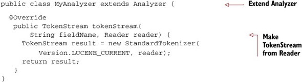
The custom analyzer tokenizes the text from the input Reader into a stream of tokens. A token is simply a word, so you can think of a text document as a stream of tokens. In listing 10.4 we’re using the StandardTokenizer to tokenize the contents on the Reader.
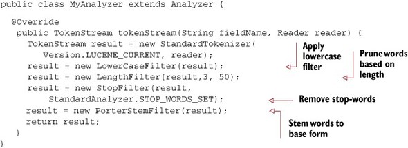
Next we try improving this Tokenizer. Instead of simply tokenizing words, we also add a filter that converts the token into lowercase. The updated class is shown in the following listing.
Listing 10.5. MyAnalyzer with lowercase filter

TokenFilter applies a transformation to the underlying token stream, and these filters can be chained. In addition to LowerCaseFilter, Lucene offers StopFilter, LengthFilter, and PorterStemFilter. StopFilter skips over stop-words in the underlying stream, LengthFilter filters out tokens whose lengths are beyond the specified range, and PorterStemFilter performs stemming on the underlying word. Stemming is a process of reducing a word into its base form. For example, the words kicked and kicking are both reduced to kick.
Note
PorterStemFilter works only for English texts, but Lucene contains stem filters for other languages too.
Using these filters, a custom Lucene Analyzer can be created, as shown in the following listing.
Listing 10.6. A custom Lucene Analyzer using multiple filters
Using this Lucene Analyzer, we can create TF-IDF vectors and cluster the data from the Reuters collections. We borrow the code from listing 9.4 and use it with this Analyzer in the following listing.
Listing 10.7. Modifying NewsKMeansClustering.java to use MyAnalyzer


This code is similar to code you saw in chapters 8 and 9. Instead of the StandardAnalyzer, we used MyAnalyzer here and ran k-means clustering over the generated vectors. After running listing 10.7’s clustering code on the Reuters data, the top 10 terms in the bank cluster look like this:
Top Terms:
                billion               =>   4.766493374867332
                bank                  =>  2.2411748607854296
                stg                   =>  1.8598368697035639
                money                =>  1.7500053112049054
                mln                   =>  1.7042239766168474
                bill                  =>  1.6742077991552187
                dlr                   =>  1.5460346601253139
                from                  =>  1.5302046415514483
                pct                   =>  1.5265302869149873
                surplus               =>  1.3873321058744208
Note that the words were stemmed using the PorterStemFilter and the StopwordsFilter has ensured that the stop-words are virtually absent. This illustrates the power of selecting the right set of features for improving clustering.
10.3.2. Writing a custom distance measure
If the vectors are of the highest quality, the biggest improvement in cluster quality comes from the choice of an appropriate distance measure. We’ve seen that the cosine distance is a good distance measure for clustering text documents. To illustrate the power of a custom distance measure, we create a different form of the cosine distance measure that exaggerates distances: it makes big distances bigger and small distances smaller. Like writing an Analyzer, writing a custom DistanceMeasure involves
- Implementing the DistanceMeasure interface
- Writing the measure in the distance(Vector v1, Vector v2) method
Our modified cosine distance measure is shown in the next listing.
Listing 10.8. A modified cosine distance measure
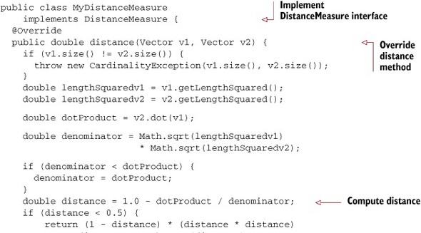

The configure (), getParameters (), and createParameters () methods are used to pass arguments to the DistanceMeasure at each job node in a MapReduce job. The method of most interest to us is the distance function. Note how it calculates the standard cosine distance measure and then tries to bring closer distances even closer by squaring the cosine distance value (if the value is between 0 and 0.5) and increases the distance otherwise.
Some interesting niche topics surfaced due to this distance measure, which were not there earlier:
Top Terms:
                futures             =>  3.2517230513480757
                trading             =>    2.73124880187049
                exchange            =>  2.2752173132458906
                market              =>  2.0752484701513274
                said                =>  1.9316076421017707
                stock               =>  1.8062251904561821
                new                 =>  1.5571645992558176
                traders             =>   1.531255338250137

                index               =>  1.3630116680911748
                options             =>   1.183384693735014
Note that this output was generated from vectors tokenized using StandardAnalyzer; you can experiment with both a custom Lucene Analyzer and a custom DistanceMeasure to get the desired clustering.
10.4. Summary
In this chapter, we explored how clustering can be improved. The algorithms, the distance measures, and the type of data all influence the output of clustering. The ClusterDumper tool can inspect output from all the clustering algorithms: the top features of each cluster and the centroid vector. This can help you understand what has happened in the clustering.
For large data sets, it’s not feasible to manually inspect all the clusters. Instead, inter-cluster and intra-cluster distances can provide a quick quantitative score of the clustering quality. If many clusters are too close, it’s time to move beyond k-means and see how partial membership and mixture distributions can be clustered out.
Writing a custom Lucene Analyzer and a custom similarity metric can help improve the clustering quality beyond what the standard implementations can do. We saw that it’s worthwhile to explore custom measures to improve clustering.
If you’ve read this far, you’re ready to take on any type of data and tune your clustering algorithm to work well. You’ll soon encounter the biggest obstacle in clustering: scale. Fortunately, Mahout can crunch terabytes of data over large Hadoop clusters. Next, we explore how the clustering algorithms in Mahout leverage the power of Hadoop. In chapter 11, you’ll see how to run a clustering job over a Hadoop cluster and take your clustering to production.