Chapter 9. Clustering algorithms in Mahout

This chapter covers

• K-means clustering
• Centroid generation using canopy clustering
• Fuzzy k-means clustering and Dirichlet clustering
• Topic modeling using latent Dirichlet allocation as a variant of clustering

Now that you know how input data is represented as Vectors and how SequenceFiles are created as input for the clustering algorithms, you’re ready to explore the various clustering algorithms that Mahout provides. There are many clustering algorithms in Mahout, and some work well for a given data set whereas others don’t. K-means is a generic clustering algorithm that can be molded easily to fit almost all situations. It’s also simple to understand and can easily be executed on parallel computers.

Therefore, before going into the details of various clustering algorithms, it’s best to get some hands-on experience using the k-means algorithm. Then it becomes easier to understand the shortcomings and pitfalls of other less generic techniques, and see how they can achieve better clustering of data in particular situations. You’ll use the k-means algorithm to cluster news articles and then improve the clustering quality using other techniques. You’ll then learn how the value of k in k-means can be inferred using canopy clustering. With this knowledge, you’ll create a clustering pipeline for a news aggregation website to get a better feel for real-world problems in clustering.

Once you’re comfortable with k-means, you’ll look at some of the shortcomings of k-means and see how other special types of clustering algorithms can be used to fill those gaps. Fuzzy k-means and Dirichlet clustering will be discussed in that context. Finally, you’ll explore latent Dirichlet allocation (LDA)—an algorithm that closely resembles clustering but that achieves something far more interesting.

There’s a lot to cover, so let’s not waste any time. Let’s jump right into the world of clustering with the k-means algorithm.

9.1. K-means clustering

K-means is to clustering as Vicks is to cough syrup. It’s a simple algorithm and it’s more than 50 years old. Stuart Lloyd first proposed the standard algorithm in 1957 as a technique for pulse code modulation, but it wasn’t until 1982 that it was published.^[1] It’s widely used as a clustering algorithm in many fields of science. The algorithm requires the user to set the number of clusters, k, as the input parameter. You’ve already seen the algorithm in action in chapter 7 when you clustered a set of points in a 2-D plane. Let’s look at the details to understand the algorithm.

¹ Stuart P. Lloyd, “Least Squares Quantization in pcm”, IEEE Transactions on Information Theory, IT-28, 2: 129–37. http://citeseerx.ist.psu.edu/viewdoc/summary?doi=10.1.1.131.1338.

The k-means algorithm puts a hard limitation on the number of clusters, k. This limitation might cause you to question the quality of this method, but fear not. This algorithm has proven to work very well for a wide range of real-world problems over the 29 years of its existence. Even if your estimate for the value k is suboptimal, the clustering quality isn’t affected much by it.

Say you’re clustering news articles to get top-level categories like politics, science, and sports. For that, you might want to choose a small value of k, perhaps in the range of 10 to 20. If fine-grained topics are needed, a larger value of k, like 50 to 100 is necessary. Suppose there are 1,000,000 news articles in your database and you’re trying to find groups of articles about the same story. The number of such related stories would be much smaller than the entire corpus—maybe in the range of 100 articles per cluster. This means you would need a k value of 10,000 to generate such a distribution. That will surely test the scalability of clustering, and this is where Mahout shines.

For good quality clustering using k-means, you’ll need to estimate a value for k. An approximate way of estimating k is to figure it out based on the data you have and the size of clusters you need. In the preceding example, where we have about a million news articles, if there are an average of 500 news articles published about every unique story, you should start your clustering with a k value of about 2,000 (1,000,000/500).

This is a crude way of estimating the number of clusters. Nevertheless, the k-means algorithm generates decent clustering even with this approximation. The type of distance measure used is the main determining factor in the quality of k-means clusters. In chapter 7, we mentioned the various kinds of distance measures in Mahout. It’s worthwhile to review them and to test their effects on the examples in this chapter.

9.1.1. All you need to know about k-means

Let’s look at the k-means algorithm in detail. Suppose we have n points that we need to cluster into k groups. The k-means algorithm will start with an initial set of k centroid points. The algorithm does multiple rounds of processing and refines the centroid locations until the iteration max-limit criterion is reached or until the centroids converge to a fixed point from which they don’t move very much.

A single k-means iteration is illustrated in figure 9.1. The actual algorithm is a series of such iterations.

No. 9

Figure 9.1. K-means clustering in action. Starting with three random points as centroids (top left), the map stage (top right) assigns each point to the cluster nearest to it. In the reduce stage (bottom left), the associated points are averaged out to produce the new location of the centroid, leaving you with the final configuration (bottom right). After each iteration, the final configuration is fed back into the same loop until the centroids come to rest at their final positions.

There are two steps in this algorithm. The first step finds the points that are nearest to each centroid point and assigns them to that specific cluster. The second step recalculates the centroid point using the average of the coordinates of all the points in that cluster.

This two-step algorithm is a classic example of an expectation maximization (EM) algorithm. In an EM algorithm, the two steps are processed repeatedly until convergence is reached. The first step, known as the expectation (E) step, finds the expected points associated with a cluster. The second step, known as the maximization (M) step, improves the estimation of the cluster center using the knowledge from the E step. A complete explanation of EM is beyond the scope of this book, but plenty of resources can be found online.^[2]

² Frank Dellaert explains the EM algorithm in terms of lower bound maximization in “The Expectation Maximization Algorithm,” http://www.cc.gatech.edu/~dellaert/em-paper.pdf. Wikipedia also has an article on the algorithm: http://en.wikipedia.org/wiki/Expectation-maximization_algorithm.

Now that you understand the k-means technique, let’s look at the important k-means classes in Mahout and run a simple clustering example.

9.1.2. Running k-means clustering

The k-means clustering algorithm is run using either the KMeansClusterer or the KMeansDriver class. The former does an in-memory clustering of the points, whereas the latter is an entry point to launch k-means as a MapReduce job. Both methods can be run like a regular Java program and can read and write data from the disk. They can also be executed on an Apache Hadoop cluster, reading data from and writing it to a distributed filesystem.

For this example, you’re going to use a random point generator function to create the points. It generates the points in Vector format as a normal distribution around a given center. You’ll cluster these points using the in-memory k-means clustering implementation in Mahout.

The generateSamples function in listing 9.1 takes a center, for example (1, 1), the standard deviation (2), and creates a set of n (400) random points around the center, which behaves like a normal distribution. You’ll similarly create two other sets with centers (1, 0) and (0, 2) and standard deviations 0.5 and 0.1 respectively. Listing 9.1 runs KMeansClusterer using the following parameters:

• The input points are in List<Vector> format.
• The DistanceMeasure is EuclideanDistanceMeasure.
• The threshold of convergence is 0.01.
• The number of clusters, k, is 3.
• The clusters were chosen using RandomPointsUtil, as in the Hello World example in chapter 7.

Listing 9.1. In-memory clustering example using the k-means algorithm

The DisplayKMeans class in Mahout’s mahout-examples module is a great tool for visualizing the algorithm in a 2-dimensional plane. It shows how the clusters shift their positions after each iteration. It’s also a great example of how clustering is done using KMeansClusterer. Run DisplayKMeans as a Java Swing application, and view the output of the example, as shown in figure 9.2.

Figure 9.2. In this example of k-means clustering we start with k set to 3 and try to cluster three normal distributions. The thin lines denote the clusters estimated in previous iterations—you can clearly see the clusters shifting.

Note that the k-means in-memory clustering implementation works with a list of Vector objects. The amount of memory used by this program depends on the total size of all the vectors. The sizes of clusters are larger than the size of the vectors in the case of sparse vectors, or they’re the same size for dense vectors. As a rule of thumb, assume that the amount of memory needed includes the total size of all of the input vectors plus the size of the k centers. If the data is huge, you can’t run this implementation.

This is where MapReduce shines. Using the MapReduce infrastructure, you can split this clustering algorithm up to run on multiple machines, with each mapper getting a subset of the points. The mapper jobs will partially compute the nearest cluster by reading the input points in a streaming fashion.

The MapReduce version of the k-means algorithm is designed to run on a Hadoop cluster, but it runs quite efficiently without one. Mahout is compiled against Hadoop code, which means you could run the same implementation without a Hadoop cluster directly from within Java and mimic Hadoop’s single machine behavior.

Understanding the K-means Clustering MapReduce Job

In Mahout, the MapReduce version of the k-means algorithm is instantiated using the KMeansDriver class. The class has just a single entry point—the runJob method.

You’ve already seen k-means in action in chapter 7. The algorithm takes the following input parameters:

• The Hadoop configuration.
• The SequenceFile containing the input Vectors.
• The SequenceFile containing the initial Cluster centers.
• The similarity measure to be used. We’ll use EuclideanDistanceMeasure as the measure of similarity and experiment with the others later.
• The convergenceThreshold. If in an iteration, the centroids don’t move more than this distance, no further iterations are done and clustering stops.
• The number of iterations to be done. This is a hard limit; the clustering stops if this threshold is reached.

Mahout algorithms never modify the input directory. This gives you the flexibility to experiment with the algorithm’s various parameters. From Java code, you can call the entry point as shown in the following listing to cluster data from the filesystem.

Listing 9.2. The k-means clustering job entry point

KmeansDriver.runJob(hadoopConf,
     inputVectorFilesDirPath, clusterCenterFilesDirPath,
     outputDir, new EuclideanDistanceMeasure(),
     convergenceThreshold, numIterations, true, false);

Tip

Mahout reads and writes data using the Hadoop FileSystem class. This provides seamless access to both the local filesystem (via java.io) and distributed filesystems like HDFS and S3FS (using internal Hadoop classes). This way, the same code that works on the local system will also work on the Hadoop filesystem on the cluster, provided the paths to the Hadoop configuration files are correctly set in the environment variables. In Mahout, the bin/mahout shell script finds the Hadoop configuration files automatically from the $HADOOP_CONF environment variable.

We’ll use the SparseVectorsFromSequenceFile tool (discussed earlier in chapter 8) to vectorize documents stored in SequenceFile to vectors. Because the k-means algorithm needs the user to input the k initial centroids, the MapReduce version similarly needs you to input the path on the filesystem where these k centroids are kept. To generate the centroid file you can write some custom logic to select the centroids, as we did in the Hello World example in listing 7.2, or you can let Mahout generate random k centroids as detailed next.

Running K-means Job using a Random Seed Generator

Let’s run k-means clustering over the vectors generated from the Reuters-21578 news collection as described in chapter 8 (section 8.3). In that chapter, the collection was converted to a Vector data set and weighted using the TF-IDF measure. The Reuters collection has many topic categories, so you’ll set k to 20 and see how k-means can cluster the broad topics in the collection.

For running k-means clustering, our mandatory list of parameters includes:

• The Reuters data set in Vector format
• The RandomSeedGenerator that will seed the initial centroids
• The SquaredEuclideanDistanceMeasure
• A large value of convergenceThreshold (1.0), because we’re using the squared value of the Euclidean distance measure
• The maxIterations set to 20
• The number of clusters, k, set to 20

If we use the DictionaryVectorizer to convert text into vectors with more than one reducer, the data set of vectors in SequenceFile format is usually found split into multiple chunks. KMeansDriver reads all the files from the input directory assuming they’re SequenceFiles. So don’t worry about the split chunks of vectors, because they’ll be taken care of by the Mahout framework.

The same is true for the folder containing the initial centroids. The centroids may be written in multiple SequenceFile files, and Mahout reads through all of them. This feature is particularly useful when you have an online clustering system where data is inserted in real time. Instead of appending to the existing file, a new chunk can be created independently and written to without affecting the algorithm.

Caution

KMeansDriver accepts an initial cluster centroid folder as a parameter. It expects a SequenceFile full of centroids only if the −k parameter isn’t set. If the -k parameter is specified, the driver class will erase the folder and write randomly selected k points to a SequenceFile there.

KMeansDriver is also the main entry point for launching the k-means clustering of the Reuters-21578 news collection. From the Mahout examples directory, execute the Mahout launcher from the shell with kmeans as the program name. This driver class will randomly select k cluster centroids using RandomSeedGenerator and then run the k-means clustering algorithm:

$ bin/mahout kmeans -i reuters-vectors/tfidf-vectors/ 
-c reuters-initial-clusters  
-o reuters-kmeans-clusters 
-dm org.apache.mahout.common.distance.SquaredEuclideanDistanceMeasure 
-cd 1.0 -k 20 -x 20 -cl

We’re using the Java execution plug-in of the Maven command to execute k-means clustering with the required command-line arguments. The –k 20 argument specifies that the centroids are randomly generated using RandomSeedGenerator and are written to the input clusters folder. The distance measure SquaredEuclideanDistanceMeasure need not be mentioned, because it’s set by default.

Tip

You can see the complete details of the command-line flags and the usage of any Mahout package by setting the –h or --help command-line flag.

Once the command is executed, clustering iterations will run one by one. Be patient and wait for the centroids to converge. An inspection of Hadoop counters printed at the end of a MapReduce can tell how many of the centroids have converged as specified by the threshold:

...
INFO: Counters: 14
May 5, 2010 2:52:35 AM org.apache.hadoop.mapred.Counters log
INFO:   Clustering
May 5, 2010 2:52:35 AM org.apache.hadoop.mapred.Counters log
INFO:     Converged Clusters=6
May 5, 2010 2:52:35 AM org.apache.hadoop.mapred.Counters log
...

Had the clustering been done in memory with the preceding parameters, it would have finished in under a minute. The same algorithm over the same data as a MapReduce job takes a couple of minutes. This increase in time is caused by the overhead of the Hadoop library. The library does many checks before starting any map or reduce task, but once they start, Hadoop mappers and reducers run at full speed. This overhead slows down the performance on a single system, but on a cluster, the negative effect of this delay is negated by the reduction in processing time due to the parallelism.

Let’s get back to the console where k-means is running. After multiple MapReduce jobs, the k-means clusters converge, the clustering ends, and the points and cluster mappings are written to the output folder.

Tip

When you deal with terabytes of data that can’t be fit into memory, the MapReduce version of the algorithm is able to scale by keeping the data on the Hadoop Distributed Filesystem (HDFS) and running the algorithm on large clusters. So if your data is small and fits in the RAM, use the in-memory implementation. If your data reaches a point where it can’t fit it into memory, start using MapReduce and think of moving the computation to a Hadoop cluster. Check out the Hadoop Quick Start tutorial at http://hadoop.apache.org/common/docs/r0.20.2/quickstart.html to find out more on setting up a pseudo-distributed Hadoop cluster on a Linux box.

The k-means clustering implementation creates two types of directories in the output folder. The clusters-* directories are formed at the end of each iteration: the clusters-0 directory is generated after the first iteration, clusters-1 after the second iteration, and so on. These directories contain information about the clusters: centroid, standard deviation, and so on. The clusteredPoints directory, on the other hand, contains the final mapping from cluster ID to document ID. This data is generated from the output of the last MapReduce operation.

The directory listing of the output folder looks something like this:

$ ls -l reuters-kmeans-clusters
drwxr-xr-x  4 user  5000  136 Feb 1 18:56 clusters-0
drwxr-xr-x  4 user  5000  136 Feb 1 18:56 clusters-1
drwxr-xr-x  4 user  5000  136 Feb 1 18:56 clusters-2
...
drwxr-xr-x  4 user  5000  136 Feb 1 18:59 clusteredPoints

Once the clustering is done, you need a way to inspect the clusters and see how they’re formed. Mahout has a utility called org.apache.mahout.utils.clustering.ClusterDumper that can read the output of any clustering algorithm and show the top terms in each cluster and the documents belonging to that cluster. To execute ClusterDumper, run the following command:

$ bin/mahout clusterdump -dt sequencefile 
-d reuters-vectors/dictionary.file-* 
-s  reuters-kmeans-clusters/clusters-19 -b 10 -n 10

The program takes the dictionary file as input. This is used to convert the feature IDs or dimensions of the Vector into words.

Running ClusterDumper on the output folder corresponding to the last iteration produces output similar to the following:

Id: 11736:
    Top Terms: debt, banks, brazil, bank, billion, he, payments, billion
     dlrs, interest, foreign
Id: 11235:
    Top Terms: amorphous, magnetic, metals, allied signal, 19.39, corrosion,
     allied, molecular, mode, electronic components
...
Id: 20073:
    Top Terms: ibm, computers, computer, att, personal, pc, operating system,
     intel, machines, dos

The reason why it’s different for different runs is that a random seed generator was used to select the k centroids. The output depends heavily on the selection of these centers. In the preceding output, the cluster with ID 11736 has top words like bank, brazil, billion, debt, and so on. Most of the articles that belong to this cluster talk about news associated with these words. Note that the cluster with ID 20073 talks about computers and related companies (ibm, att, pc, and so on).

As you can see, you’ve achieved a decent clustering using a distance measure like SquaredEuclideanDistanceMeasure, but it took more than 10 iterations to get there. What’s peculiar about text data is that two documents that are similar in content don’t necessarily need to have the same length. The Euclidean distance between two documents of different sizes and similar topics is quite large. That is, the Euclidean distance is affected more by the difference in the number of words between the two documents, and less by the words common to both of them. To better understand this, revisit section 7.4.1 and see the Euclidean distance equation’s behavior by experimenting with it.

These reasons make Euclidean distance measurement a misfit for text documents. Take a look at this cluster that was created with the Euclidean distance metric:

Id: 20978:
    Top Terms: said, he, have, market, would, analysts, he said, from, which,
     has

This cluster really doesn’t make any sense, especially with words like said, he, and the. To really get good clustering for a given data set, you have to experiment with the different distance measures available in Mahout, as discussed in section 7.4, and see how they perform on the data you have.

You’ve read that the Cosine distance and Tanimoto measures work well for text documents because they depend more on common words and less on uncommon words. To see this in action, we’ll experiment with the Reuters data set and compare the output with the output of the previous clustering. Let’s run k-means with CosineDistanceMeasure:

$ bin/mahout kmeans -i reuters-vectors/tfidf-vectors/ 
-c reuters-initial-clusters  
-o reuters-kmeans-clusters 
-dm org.apache.mahout.common.distance.CosineDistanceMeasure 
-cd 0.1 -k 20 -x 20 -cl

Note that this example sets the convergence threshold to 0.1, instead of using the default value of 0.5, because cosine distances lie between 0 and 1. When the program runs, one peculiar behavior is noticeable: the clustering speed slows down a bit due to the extra calculation involved in cosine distances, but the clustering converges within a few iterations as compared to over 10 when using the squared Euclidean distance measure. This clearly indicates that cosine distance gives a better notion of similarity between text documents than Euclidean distance.

Once the clustering finishes, we can run the ClusterDumper against the output and inspect some of the top words in each cluster. These are some of the interesting clusters:

Id: 3475:name:
    Top Terms: iranian, iran, iraq, iraqi, news agency, agency, news, gulf,
     war, offensive
Id: 20861:name:
    Top Terms: crude, barrel, oil, postings, crude oil, 50 cts, effective,
     raises, bbl, cts

Experiment with Mahout’s k-means algorithm and find the combination of DistanceMeasure and convergenceThreshold that gives the best clustering for the given problem. Try it on various kinds of data and see how things behave. Explore the various distance measures in Mahout, or try to make one on your own. Though k-means runs impeccably well using randomly seeded clusters, the final centroid locations still depend on their initial positions.

The k-means algorithm is an optimization technique. Given the initial conditions, k-means tries to put the centers at their optimal positions. But it’s a greedy optimization that causes it to find the local minima. There can be other centroid positions that satisfy the convergence property, and some of them might be better than the results we just got. We may never find the perfect clusters, but we can apply one powerful technique that will take us closer to it.

9.1.3. Finding the perfect k using canopy clustering

For many real-world clustering problems, the number of clusters isn’t known beforehand, like the grouping of books in the library example from chapter 7. A class of techniques known as approximate clustering algorithms can estimate the number of clusters as well as the approximate location of the centroids from a given data set. One such algorithm is called canopy generation.

The k-means implementation in Mahout by default generates the SequenceFile containing k vectors using the RandomSeedGenerator class. Although random centroid generation is fast, there’s no guarantee that it will generate good estimates for centroids of the k clusters. Centroid estimation greatly affects the run time of k-means. Good estimates help the algorithm to converge faster and use fewer passes over the data. Automatically finding the number of clusters just by looking at the data is exciting, but the canopy algorithm still has to be told what size clusters to look for, and it will find the number of clusters that have approximately that size.

Seeding K-means Centroids using Canopy Generation

Canopy generation, also known as canopy clustering, is a fast approximate clustering technique. It’s used to divide the input set of points into overlapping clusters known as canopies. The word canopy, in this context, refers to an enclosure of points, or a cluster. Canopy clustering tries to estimate the approximate cluster centroids (or canopy centroids) using two distance thresholds.

Canopy clustering’s strength lies in its ability to create clusters extremely quickly—it can do this with a single pass over the data. But its strength is also its weakness. This algorithm may not give accurate and precise clusters. But it can give the optimal number of clusters without even specifying the number of clusters, k, as required by k-means.

The algorithm uses a fast distance measure and two distance thresholds, T₁ and T₂, with T₁ > T₂. It begins with a data set of points and an empty list of canopies, and then iterates over the data set, creating canopies in the process. During each iteration, it removes a point from the data set and adds a canopy to the list with that point as the center. It loops through the rest of the points one by one. For each one, it calculates the distances to all the canopy centers in the list. If the distance between the point and any canopy center is within T₁, it’s added into that canopy. If the distance is within T₂, it’s removed from the list and thereby prevented from forming a new canopy in the subsequent loops. It repeats this process until the list is empty.

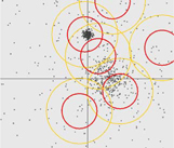
This approach prevents all points close to an already existing canopy (distance < T₂) from being the center of a new canopy. It’s detrimental to form another redundant canopy in close proximity to an existing one. Figure 9.3 illustrates the canopies created using this method. Which clusters are formed depends only on the choice of distance thresholds.

Figure 9.3. Canopy clustering: if you start with a point (top left) and mark it as part of a canopy, all the points within distance T₂ (top right) are removed from the data set and prevented from becoming new canopies. The points within the outer circle (bottom-right) are also put in the same canopy, but they’re allowed to be part of other canopies. This assignment process is done in a single pass on a mapper. The reducer computes the average of the centroid (bottom right) and merges close canopies.

Understanding the Canopy Generation Algorithm

The canopy generation algorithm is executed using the CanopyClusterer or the CanopyDriver class. The former does in-memory clustering of the points, whereas the latter implements it as MapReduce jobs. These jobs can be run like a regular Java program and can read and write data from the disk. They can also be run on a Hadoop cluster, reading data from and writing it to a distributed filesystem.

We’re going to use the same random point generator function as earlier to create vectors scattered in the 2-dimensional plane, like in a normal distribution. For this example, we’ll generate three normal distributions. Listing 9.3 runs the in-memory version of canopy clustering using the CanopyClusterer with the following parameters:

• The input Vector data is in List<Vector> format.
• The DistanceMeasure is EuclideanDistanceMeasure.
• The value of T₁ is 3.0.
• The value of T₂ is 1.5.

Listing 9.3. In-memory example of the canopy generation algorithm

The DisplayCanopy class in Mahout’s mahout-examples module displays a set of points in a 2-dimensional plane and shows how the canopy generation is done using the in-memory CanopyClusterer. Typical output of DisplayCanopy is shown in figure 9.4.

Figure 9.4. An example of in-memory canopy generation visualized using the DisplayCanopy class, that’s included in examples bundled with Mahout. We started with T₁ = 3.0 and T₂ = 1.5 and clustered the randomly generated points.

Canopy clustering doesn’t require you to specify the number of cluster centroids as a parameter. The number of centroids formed depends only on the choice of the distance measures, T₁ and T₂. The in-memory canopy clustering implementation works with a list of Vector objects, just like the k-means implementation. If the data set is huge, it’s not possible to run this algorithm on a single machine, and the MapReduce job is required. The MapReduce version of the canopy clustering implementation does a slight approximation as compared to the in-memory one and produces a slightly different set of canopies for the same input data. This is nothing to be alarmed about when the data is huge. The output of canopy clustering is a great starting point for k-means, which improves clustering due to the increased precision of the initial centroids as compared to random selection.

Using the canopies you’ve generated, you can assign points to the nearest canopy centers, in theory clustering the set of points. This is called canopy clustering instead of canopy generation. In Mahout, the CanopyDriver class does canopy centroid generation and optionally also clusters the points if the runClustering parameter is set to true.

Next, you’ll run canopy generation on the Reuters collection and figure out the value of k.

Running the Canopy Generation Algorithm to Select k Centroids

Let’s now generate canopy centroids from the Reuters Vector data set. To generate the centroids, you’ll set the distance measure to EuclideanDistanceMeasure and use threshold values of t1=2000 and t2=1500. Remember that the Euclidean distance measure gives very large distance values for sparse document vectors, so large values for t1 and t2 are necessary to get meaningful clusters.

The distance threshold values (t1 and t2) selected in this case produce less than 50 centroid points for the Reuters collection. We estimated these threshold values after running the CanopyDriver multiple times over the input data. Due to the fast nature of canopy clustering, it’s possible to experiment with various parameters and see the results much more quickly than when using expensive techniques like k-means.

To run canopy generation over the Reuters data set, execute the canopy program using the Mahout launcher as follows:

$ bin/mahout canopy -i reuters-vectors/tfidf-vectors 
-o reuters-canopy-centroids 
-dm org.apache.mahout.common.distance.EuclideanDistanceMeasure 
-t1 1500 -t2 2000

Within a minute, CanopyDriver will generate the centroids in the output folder. You can inspect the canopy centroids using the cluster dumper utility, as you did for k-means earlier in this chapter.

Next, we’ll use this set of centroids to improve k-means clustering.

Improving K-means Clustering using Canopy Centers

We can now run the k-means clustering algorithm using the canopy centroids generated in the previous section. For that, all we need to do is set the clusters parameter (-c) to the canopy clustering output folder and remove the –k command-line parameter in KMeansDriver. (Be careful: if the –k flag is set, the RandomSeedGenerator will overwrite the canopy centroid folder.)

We’ll use TanimotoDistanceMeasure in k-means to get clusters as follows:

$ bin/mahout kmeans -i reuters-vectors/tfidf-vectors 
-o reuters-kmeans-clusters 
-dm org.apache.mahout.common.distance.TanimotoDistanceMeasure  
-c reuters-canopy-centroids/clusters-0 -cd 0.1 -ow -x 20 -cl

After the clustering is done, use ClusterDumper to inspect the clusters. Some of them are listed here:

Id: 21523:name:
     Top Terms:
tones, wheat, grain, said, usda, corn, us, sugar, export, agriculture
Id: 21409:name:
     Top Terms:
stock, share, shares, shareholders, dividend, said, its, common, board,
     company
Id: 21155:name:
     Top Terms:
oil, effective, crude, raises, prices, barrel, price, cts, said, dlrs
Id: 19658:name:
     Top Terms:
drug, said, aids, inc, company, its, patent, test, products, food
Id: 21323:name:
     Top Terms:
        7-apr-1987, 11, 10, 12, 07, 09, 15, 16, 02, 17

Note the last cluster. Although the others seem to be great topic groups, the last one looks meaningless. Nevertheless, the clustering grouped documents with these terms because the terms occur together in these documents. Another issue is that words like its and said in these clusters are useless from a language standpoint. The algorithm simply doesn’t know that. Any clustering algorithm can generate good clustering provided the highest weighted features of the vector represent good features of the document.

In sections 8.3 and 8.4, you saw how TF-IDF and normalization gave higher weights to the important features and lower weights to the stop-words, but occasionally spurious clusters do surface. A quick and effective way to avoid this problem is to remove these words from ever occurring as features in the document Vector. In the next case study, you’ll see how to fix this by using a custom Lucene Analyzer class.

Canopy clustering is a good approximate clustering technique, but it suffers from memory problems. If the distance thresholds are close, too many canopies are generated, and this increases memory usage in the mapper. This might exceed available memory while running on a large data set with a bad set of thresholds. The parameters need to be tuned to fit the data set and the clustering problem, as you’ll see next.

The next example we’ll look at creates a clustering module for a news website. We chose a news website because it best represents a dynamic system where content needs to be organized with very good precision. Clustering can help solve the issues related to such content systems.

9.1.4. Case study: clustering news articles using k-means

In this case study, we’re going to assume that we’re in charge of a fictional news aggregation website called AllMyNews.com. A user who comes to the website uses keywords to search for the content they’re looking for. If they see an interesting article, they can use the words in the article to search for related articles, or they can drill down into the news category and explore related news articles there. Usually we rely on human editors to find related items and help categorize and cross-link the whole website. But if articles are coming in at tens of thousands per day, human intervention might prove too expensive. Enter clustering.

Using clustering, we may be able to find related stories automatically and be able to give the user a better browsing experience. In this section, you’ll use k-means clustering to implement such a feature. Look at figure 9.5 for an example of what the feature should look like in practice. For a news story on the website, we’ll show the user a list of all related news articles.

Figure 9.5. An example of related-articles functionality taken from the Google News website. The links to similar stories within the cluster are shown at the bottom in bold. The top related articles are shown as links above that.

For any given article, we can store the cluster in which the articles reside. When a user requests articles related to the one they’re reading, we’ll pick out all the articles in the cluster, sort them based on the distance to the given article, and present them to the user.

That’s a great initial design for a news-clustering system, but it doesn’t solve all the issues completely. Let’s list some real-life problems we might face in such a context:

• There are articles coming in every minute, and the website needs to refresh its clusters and indexes.
• There might be multiple stories breaking out at the same time, so we’ll require separate clusters for them, which means we need to add more centroids every time this happens.
• The quality of the text content is questionable, because there are multiple sources feeding in the data. We need to have mechanisms to clean up the content when doing feature selection.

We’ll start with an efficient k-means clustering implementation to cluster the news articles offline. Here, the word offline means we’ll write the documents into SequenceFiles and start the clustering as a backend process. We won’t go into the details of how the news data is stored. We’ll assume for simplicity that document storage and retrieval blocks can’t be replaced easily by database read/write code.

Note

In the coming chapters, we’ll modify this case study and add advanced techniques using Mahout to solve issues related to speed and quality. Finally, in chapter 12 we’ll show a working, tuned, and scalable clustering example applied to some real-world datasets that can be adapted for different applications.

Listing 9.4 shows the code that clusters news articles from SequenceFiles, and listing 9.5 shows a custom Lucene Analyzer class that prunes away non-alphabetic features from the data.

Listing 9.4. News clustering using canopy generation and k-means clustering

Listing 9.5. A custom Lucene analyzer that filters non-alphabetic tokens

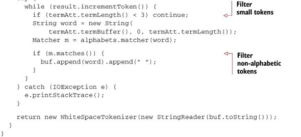
This NewsKMeansClustering example is straightforward. The documents are stored in the input directory. From these, we create vectors from unigrams and bigrams that contain only alphabetic characters. Using the generated Vectors as input, we run the canopy centroid generation job to create the seed set of centroids for the k-means clustering algorithm. Finally, at the end of k-means clustering, we read the output and save it to the database.

The next section looks at the other algorithms in Mahout that can take us further than k-means.

9.2. Beyond k-means: an overview of clustering techniques

K-means produces rigid clustering. For example, a news article that talks about the influence of politics in biotechnology could be clustered either with the politics documents or with the biotechnology documents, but not with both. Because we’re trying to tune the related-articles feature, we might need overlapping or fuzzy information. We might also need to model the point distribution of our data, and this isn’t something k-means was designed to do.

K-means is just one type of clustering. There are many other clustering algorithms designed on different principles, which we’ll look at next.

9.2.1. Different kinds of clustering problems

Recall that clustering is simply a process of putting things into groups. To do more than simple grouping, you need to understand the different kinds of problems in clustering. These problems and their solutions fall mainly into four categories:

• Exclusive clustering
• Overlapping clustering
• Hierarchical clustering
• Probabilistic clustering

Let’s look at each in turn.

Exclusive Clustering

In exclusive clustering, an item belongs exclusively to one cluster, not several. Recall the discussion about clustering books in a library from chapter 7. We could have simply associated a book like Harry Potter only with the cluster of fiction books. Thus, Harry Potter would have exclusively belonged to the fiction cluster. K-means does this sort of exclusive clustering, so if the clustering problem demands this behavior, k-means will usually do the trick.

Overlapping Clustering

What if we wanted to do non-exclusive clustering; that is, put Harry Potter not only in fiction but also in a young adult cluster as well as under fantasy. An overlapping clustering algorithm like fuzzy k-means achieves this easily. Moreover, fuzzy k-means also indicates the degree with which an object is associated with a cluster. Harry Potter might be inclined more towards the fantasy cluster than the young adult cluster. The difference between exclusive and overlapping clustering is illustrated in figure 9.6.

Figure 9.6. Exclusive clustering versus overlapping clustering with two centers. In the former, squares and triangles each have their own cluster, and each belongs only to one cluster. In overlapping clustering, some shapes, like pentagons, can belong to both clusters with some probability, so they’re part of both clusters instead of having a cluster of their own.

Hierarchical Clustering

Now, assume a situation where we have two clusters of books, one for fantasy and the other for space travel. Harry Potter is in the cluster of fantasy books, but these two clusters, space travel and fantasy, could be visualized as subclusters of fiction. Hence, we can construct a fiction cluster by merging these and other similar clusters. The fiction and fantasy clusters have a parent-child relationship, as illustrated in figure 9.7, and hence the name hierarchical clustering.

Figure 9.7. Hierarchical clustering: a bigger cluster groups two or more smaller clusters in the form of a tree-like hierarchy. Recall the library example in chapter 7—we did a crude form of hierarchical clustering when we simply stacked books based on the similarity between them.

Similarly, we could keep grouping clusters into bigger and bigger ones. At a certain point, the clusters would be so large and so generic that they’d be useless as groupings. Nevertheless, this is a useful method of clustering: merging small clusters until it becomes undesirable to do so. Methods that uncover such a systematic tree-like hierarchy for a given data collection are called hierarchical clustering algorithms.

Probabilistic Clustering

A probabilistic model is usually a characteristic shape or a type of distribution of a set of points in an n-dimensional plane. There are a variety of probabilistic models that fit known data patterns. Probabilistic clustering algorithms try to fit a probabilistic model over a data set and adjust the model’s parameters to correctly fit the data. Such correct fits rarely happen; instead, these algorithms give a percentage match or a probability value, which indicates how well the model fits the cluster.

To explain how this fitting happens, look at the 2-dimensional example in figure 9.8. Say that we somehow know that all points in a plane are distributed in various regions with an elliptical shape, but we don’t know the center and radius or axes of these regions. We’ll choose an elliptical model and try to fit it to the data; we’ll move, stretch, or contract each ellipse to best fit a region and do this for all the regions. This is called model-based clustering.

Figure 9.8. A simplified view of probabilistic clustering. The initial set of points is on the left. On the right, the first set of points matches an elongated elliptical model whereas the second one is more symmetric.

A typical example of this type is the Dirichlet clustering algorithm, which does the fitting based on a model provided by the user. We’ll see this clustering algorithm in action in section 9.4. Before we get there, though, you need to understand how different clustering algorithms are grouped based on their strategies.

9.2.2. Different clustering approaches

Different clustering algorithms take different approaches. We can categorize most of these approaches as follows:

• Fixed number of centers
• Bottom-up approach
• Top-down approach

There are many other clustering algorithms that have unique ways of clustering, but you may never encounter them in Mahout, because they currently aren’t scalable on large data sets. Instead, we’ll explore the algorithms in those three categories.

Fixed Number of Centers

These clustering methods fix the number of clusters ahead of time. The count of clusters is typically denoted by the letter k, which originated from the k of the k-means algorithm, which is the best known of these methods. The idea is to start with k and to modify these k cluster centers to better fit the data. Once the centers have converged to match the data, the points in the data set are assigned to the centroid closest to them.

Fuzzy k-means is another example of an algorithm that requires a fixed number of clusters. Unlike k-means, which does exclusive clustering, fuzzy k-means does overlapping clustering.

Bottom-Up Approach: From Points to Clusters Via Grouping

When you have a set of points in n-dimensions, you can do two things: assume that all points belong to a single cluster and start dividing the cluster into smaller clusters, or assume that each of the data point begins in its own cluster and start grouping them iteratively. The former is a top-down approach and the latter is a bottom-up approach.

The bottom-up clustering algorithms work as follows: from a set of points in an n-dimensional space, the algorithm finds the pairs of points close to each other and merges them into one cluster, as illustrated in figure 9.9. This merge is done only if the distance between them is below a certain threshold value. If not, those points are left alone. This process of merging the clusters using the distance measure is repeated until nothing can be merged anymore.

Figure 9.9. Bottom-up clustering: After every iteration the clusters are merged to produce larger and larger clusters until it’s not feasible to merge based on the given distance measure.

Top-Down Approach: Splitting the Giant Cluster

In the top-down approach, you start with assigning all points to a single giant cluster. Then you find the best possible way to split this giant cluster into two smaller clusters, as illustrated in figure 9.10. These clusters are divided repeatedly until you get clusters that are meaningful, based on some distance measure criterion.

Figure 9.10. Top-down clustering: during each iteration, the clusters are divided into two by finding the best splitting until you get the clusters you desire.

Though this is straightforward, finding the best possible split for a set of n-dimensional points isn’t easy. Moreover, most of these algorithms can’t be easily reduced into the MapReduce form, so they aren’t currently available in Mahout.

An example of a top-down algorithm is spectral clustering. In spectral clustering, the splitting is decided by finding the line or plane that cuts the data into two sets with a larger margin between the two sets.

Advantages and Disadvantages of the Top-Down and Bottom-Up Approaches

The beauty of the top-down and bottom-up approaches is that they don’t require the user to input the cluster size. This means that in a data set where the distribution of the points is unclear, both these types of algorithms output clusters based solely on the similarity metric. This works quite well in many applications.

These approaches are still being researched and they can’t be run as MapReduce jobs. But even though Mahout has no implementations of these methods, other specialized algorithms implemented in Mahout can run as MapReduce jobs without specifying the number of clusters.

The lack of hierarchical clustering algorithms in MapReduce is easily circumvented by the smart use of k-means, fuzzy k-means, and Dirichlet clustering. To get the hierarchy, start with a small number of clusters (k) and repeat clustering with increasing values of k. Alternatively, you can start with a large number of centroids and start clustering the cluster centroids with decreasing values of k. This mimics the hierarchical clustering behavior while making full use of the scalable nature of Mahout implementations.

The next section deals with the fuzzy k-means algorithm in detail. We use it to improve our clustering of related articles for our news website, AllMyNews.com.

9.3. Fuzzy k-means clustering

As the name says, the fuzzy k-means clustering algorithm does a fuzzy form of k-means clustering. Instead of the exclusive clustering in k-means, fuzzy k-means tries to generate overlapping clusters from the data set. In the academic community, it’s also known as the fuzzy c-means algorithm. You can think of it as an extension of k-means.

K-means tries to find the hard clusters (where each point belongs to one cluster) whereas fuzzy k-means discovers the soft clusters. In a soft cluster, any point can belong to more than one cluster with a certain affinity value towards each. This affinity is proportional to the distance from the point to the centroid of the cluster. Like k-means, fuzzy k-means works on those objects that can be represented in n-dimensional vector space and it has a distance measure defined.

9.3.1. Running fuzzy k-means clustering

The fuzzy k-means algorithm is available in the FuzzyKMeansClusterer and FuzzyKMeansDriver classes. The former is an in-memory implementation, and the latter uses MapReduce.

Let’s look at an example. You’ll use the same random point generator function you used earlier to scatter points in a 2-dimensional plane. Listing 9.6 shows the in-memory implementation using FuzzyKMeansClusterer with the following parameters:

• The input Vector data is in List<Vector> format.
• The DistanceMeasure is EuclideanDistanceMeasure.
• The threshold of convergence is 0.01.
• The number of clusters, k, is 3.
• The fuzziness parameter, m, is 3. (This parameter will be explained in section 9.3.2.)

Listing 9.6. In-memory example of fuzzy k-means clustering

The DisplayFuzzyKMeans class in Mahout’s mahout-examples module is a good tool for visualizing this algorithm on a 2-dimensional plane. DisplayFuzzyKMeans runs as a Java Swing application and produces output like that shown in figure 9.11.

Figure 9.11. Fuzzy k-means clustering: the clusters look like they’re overlapping each other, and the degree of overlap is decided by the fuzziness parameter.

MapReduce Implementation of Fuzzy K-means

The MapReduce implementation of fuzzy k-means looks similar to that of the k-means implementation in Mahout. These are the important parameters:

• The input data set in Vector format.
• The RandomSeedGenerator to seed the initial k clusters.
• The distance measure: SquaredEuclideanDistanceMeasure in this case.
• A large value of convergenceThreshold, such as –cd 1.0, because we’re using the squared value of the distance measure.
• A value for maxIterations; we’ll use the default value of –x 10.
• The coefficient of normalization, or the fuzziness factor, with a value greater than –m 1.0; this will be explained in the section 9.3.2.

To run the fuzzy k-means clustering over the input data, use the Mahout launcher with the fkmeans program name as follows:

$ bin/mahout fkmeans 
-i reuters-vectors/tfidf-vectors/ -c reuters-fkmeans-centroids 
-o reuters-fkmeans-clusters -cd 1.0 -k 21 -m 2 -ow -x 10
-dm org.apache.mahout.common.distance.SquaredEuclideanDistanceMeasure

As with k-means, FuzzyKMeansDriver will automatically run the RandomSeedGenerator if the number of clusters (-k) flag is set. Once the random centroids are generated, fuzzy k-means clustering will use them as the input set of k centroids. The algorithm runs multiple iterations over the data set until the centroids converge, each time creating the output in the cluster-folder. Finally, it runs another job that generates the probabilities of each point belonging to a particular cluster based on the distance measure and the fuzziness parameter (-m).

Before we get into the details of the fuzziness parameter, it’s a good idea to inspect the clusters using the ClusterDumper tool. ClusterDumper shows the top words of the cluster for each centroid. To get the actual mapping of the points to the clusters, you need to read the SequenceFiles in the clusteredPoints/folder. Each entry in the sequence file has a key, which is the identifier of the vector, and a value, which is the list of cluster centroids with an associated numerical value, which indicates how well the point belongs to that particular centroid.

9.3.2. How fuzzy is too fuzzy?

Fuzzy k-means has a parameter, m, called the fuzziness factor. Like k-means, fuzzy k-means loops over the data set but instead of assigning vectors to the nearest centroids, it calculates the degree of association of the point to each of the clusters.

Suppose for a vector, V, that d₁, d₂, ... d_k are the distances to each of the k cluster centroids. The degree of association (u1) of vector (V) to the first cluster (C₁) is calculated as

Similarly, you can calculate the degree of association to other clusters by replacing d₁ in the numerators of the denominator expression with d₂, d₃, and so on. It’s clear from the expression that m should be greater than 1, or else the denominator of the fraction becomes 0 and things break down.

If you choose a value of 2 for m, you’ll see that all degrees of association for any point sum up to one. If, on the other hand, m comes very close to 1, like 1.000001, more importance will be given to the centroid closest to the vector. The fuzzy k-means algorithm starts behaving more like the k-means algorithm as m gets closer to 1. If m increases, the fuzziness of the algorithm increases, and you’ll begin to see more and more overlap.

The fuzzy k-means algorithm also converges better and faster than the standard k-means algorithm.

9.3.3. Case study: clustering news articles using fuzzy k-means

The related-articles functionality will certainly be richer with partial overlap of clusters. The partial score will help us rank the related articles according to their relatedness to the cluster. In the following listing, the case study example from section 9.1.4 is modified to use the fuzzy k-means algorithm and retrieve the fuzzy cluster membership information.

Listing 9.7. News clustering using fuzzy k-means clustering

The fuzzy k-means algorithm gives us a way to refine the related-articles code. Now we know by what degree a point belongs to a cluster. Using this information, we can find the top clusters a point belongs to, and use the degree to find the weighted score of articles. This way we avoid the strictness of exclusive clustering and identify better-related articles for documents lying on the boundaries of a cluster.

9.4. Model-based clustering

The complexities of clustering algorithms have increased progressively in this chapter. We started with k-means, a fast clustering algorithm. Then we captured partial clustering membership using fuzzy k-means. We also optimized the clustering using centroid generation algorithms like canopy clustering.

What more do we want to know about these clusters? To better understand the structures within the data, we may need a method that’s completely different from the algorithms we’ve discussed so far—model-based clustering methods.

Before we focus on what model-based clustering is, we need to look at some of the issues faced by k-means and other related algorithms. One such method is Dirichlet process clustering, and we’ll be dealing with it throughout this section. But to understand it, you need to first understand what kind of problems it solves, and the best way to do that is to compare it to the clustering algorithms you’ve already seen in this chapter. So we’ll look at what k-means can’t do, and then see how Dirichlet process clustering solves that problem.

9.4.1. Deficiencies of k-means

Say you wanted to cluster a data set into k clusters. You’ve learned how to run k-means and get the clusters quickly. K-means works well because it can easily divide clusters using a linear distance.

What if you knew that the clusters were based on a normal distribution and are mixed together and overlap each other? Here, you might be better off with fuzzy k-means clustering.

What if the clusters themselves aren’t in a normal distribution? What if the clusters have an ovoid shape? Neither k-means nor fuzzy k-means knows how to use this information to improve the clustering. Before we look at how to solve this problem, let’s first look at an example where k-means clustering fails to describe a simple distribution of data.

Asymmetrical Normal Distribution

You’re going to run k-means clustering using points generated from an asymmetrical normal distribution. What this means is that instead of the points being scattered in two dimensions around a point in a circular area, you’re going to make the point-generator generate clusters of points having different standard deviations in different directions. This creates an ellipsoidal area in which the points are concentrated. We’ll then run the in-memory k-means implementation over this data.

Figure 9.12 shows the ellipsoidal or asymmetric distribution of points and the clusters generated by k-means. It’s clear that k-means isn’t powerful enough to figure out the distribution of these points.

Figure 9.12. Running k-means clustering over an asymmetric normal distribution of points. The points are scattered in an oval area instead of a circular one. K-means can’t generate a perfect fit for the data.

Another issue with k-means is that it requires you to estimate k, the number of seed centroids, and this value is usually overestimated. Finding the optimal value of k isn’t easy unless you have a clear understanding of the data, which happens rarely. Even by doing canopy generation, you need to tune the distance measure to make the algorithm improve the estimate of k.

What if there was a better way to find the number of clusters? That’s where model-based clustering proves to be useful.

Issues with Clustering Real-World Data

Suppose we want to cluster a population of people based on their movie preferences to find like-minded people. We could estimate the number of clusters in such a population by counting the different genres of movies.

Some of the clusters we’d find are people who like action movies, people who like romantic movies, people who like comedies, and so on. This isn’t a good estimation, though, because there are tons of exceptions. For example, there are clusters of people who like only gangster movies, not other action movies. They form a subcluster within the action cluster. With such a complex mixing of clusters, we’ll never get the information about a small cluster because a bigger cluster would always subsume it. The only way to improve this situation is to somehow understand that a population’s movie preferences are hierarchical in nature.

If we had known this earlier, we’d have used a hierarchical clustering method to better cluster the people. But those methods can’t capture the overlap. None of the clustering algorithms we’ve seen so far can capture the hierarchy and the overlap at the same time. What method can we use to uncover this information?

That’s another thing that’s tackled by model-based clustering.

9.4.2. Dirichlet clustering

Mahout has a model-based clustering algorithm: Dirichlet clustering. The name Dirichlet refers to a family of probability distributions defined by a German mathematician, Johann Peter Gustav Lejeune Dirichlet. Dirichlet clustering performs something known as mixture modeling using calculations based on the Dirichlet distribution.

The whole process might sound complicated without a deeper understanding of Dirichlet distributions, but the idea is simple. Say you know that your data points are concentrated in an area like a circle and they’re well distributed within it, and you also have a model that explains this behavior. You can test whether your data fits the model by reading through the vectors and calculating the probability of the model being a fit to the data.

This approach can say with some degree of confidence that the concentration of points looks more like a circular model. It can also say that the region looks less like a triangle, another model, due to lesser probability of the data matching the triangle. If you find a fit, you know the structure of your data. Figure 9.13 illustrates this concept. (Note that circles and triangles are used here just for visualizing this algorithm. They aren’t to be mistaken for the real probabilistic models on which this algorithm works.)

Figure 9.13. Dirichlet clustering: the models are made to fit the given data set as best they can to describe it. The right model will fit the data better and indicates the number of clusters in the data set that correlates with the model.

Dirichlet clustering is implemented as a Bayesian clustering algorithm in Mahout. That means the algorithm doesn’t just want to give one explanation of the data; rather, it wants to give lots of explanations. This is like saying, “Region A is like a circle, region B is like a triangle, together regions A and B are like a polygon,” and so on. In reality, these regions are statistical distributions, like the normal distribution that you saw earlier in the chapter.

We’ll look at various model distributions a little later in this section, but a full discourse on them is beyond the scope of this book. First, though, let’s look at how the Dirichlet clustering implementation in Mahout works.

Understanding the Dirichlet Clustering Algorithm

Dirichlet clustering starts with a data set of points and a ModelDistribution. Think of ModelDistribution as a class that generates different models. You create an empty model and try to assign points to it. When this happens, the model crudely grows or shrinks its parameters to try and fit the data. Once it does this for all points, it re-estimates the parameters of the model precisely using all the points and a partial probability of the point belonging to the model.

At the end of each pass, you get a number of samples that contain the probabilities, models, and assignment of points to models. These samples could be regarded as clusters, and they provide information about the models and their parameters, such as their shape and size. Moreover, by examining the number of models in each sample that have some points assigned to them, you can get information about how many models (clusters) the data supports. Also, by examining how often two points are assigned to the same model, you can get an approximate measure of how likely these points are to be explained by the same model. Such soft-membership information is a side product of using model-based clustering. Dirichlet clustering is able to capture the partial probabilities of points belonging to various models.

9.4.3. Running a model-based clustering example

Dirichlet process-based clustering is implemented in memory in the DirichletClusterer class and as a MapReduce job in DirichletDriver. We’re going to use the generateSamples function (used earlier in section 9.1.2) to create random vectors.

The Dirichlet clustering implementation is generic enough to use with any type of distribution and any data type. The Model implementations in Mahout use the VectorWritable type, so we’ll be using that as the default type in our clustering code.

We’ll run the Dirichlet clustering using the following parameters:

• The input Vector data is in List<VectorWritable> format.
• The GaussianClusterDistribution is the model distribution we’ll try to fit our data to.
• The alpha value of the Dirichlet distribution is 1.0.
• The number of models (numModels) we’ll start with is 10.
• The thin and burn intervals are 2 and 2.

The points will be scattered around a specified center point like a normal distribution, as shown in the following listing.

Listing 9.8. Dirichlet clustering using normal distribution

In listing 9.8, we generate some sample points using a normal distribution and try to fit the normal (Gaussian) model distribution over the data. The parameters of the algorithm determine the speed and quality of convergence.

Here, alpha is a smoothing parameter. A higher value slows down the speed of convergence of the model, so the clustering will have many iterations and will try to overfit the models (the model will find a fitting distribution of data in a smaller area, even if the larger area is the model we may be trying to find). A lower value causes the clustering to merge models more quickly and hence tries to under-fit the model (to create models from points that could ideally have been from two different distributions).

The thin and the burn intervals are used to decrease the memory usage of the clustering. The burn parameter specifies how many iterations to complete before saving the first set of models for the data set. The thin parameter decides how many iterations to skip between saving such a model configuration. Many iterations are needed to reach convergence, and the initial states aren’t worth exploring. During the initial stages, the number of models is extremely high and they provide no real value, so we can skip them (with thin and burn) to save memory.

The final state achieved using the DisplayDirichlet clustering example is shown in figure 9.14. This class can be found in Mahout’s examples folder along with examples of plenty of other model distributions and their clustering.

Figure 9.14. Dirichlet clustering with a normal distribution using the DisplayDirichlet class in the Mahout examples folder

The kind of clusters we got here are different from the output of the k-means clustering in section 9.2. Dirichlet clustering did something that k-means couldn’t do, which was to identify the three clusters exactly the way we generated them. Any other algorithm would have just tried to cluster things into overlapping or hierarchical groups.

This is just the tip of the iceberg. To show off the awesome power of model-based clustering, we repeat this example with something more difficult than a normal distribution.

Asymmetric Normal Distribution

A normal distribution is asymmetrical when the standard deviations of points along different dimensions are different. This gives it an ellipsoidal shape. When you ran k-means clustering on this distribution in section 9.4.1, it broke down miserably. Now you’ll attempt to cluster the same set of points using Dirichlet clustering with GaussianClusterDistribution, by keeping the parameters different for x- and y-axes.

You’ll run Dirichlet clustering using the asymmetric normal model on the set of 2-dimensional points that has different standard deviations along the x and y directions. The output of the clustering is shown in figure 9.15.

Figure 9.15. Dirichlet clustering with asymmetrical normal distribution illustrated using the DisplayDirichlet code in the Mahout examples folder. The thick oval lines denote the final state, and the thinner lines are the states in previous iterations.

Even though the number of clusters formed seems to have increased, model-based clustering was able to find the asymmetric model and fit the model to the data much better than any of the other algorithms. A better value of alpha might have improved this.

Next, we experiment with the MapReduce version of Dirichlet clustering.

MapReduce Version of Dirichlet Clustering

Like other implementations in Mahout, Dirichlet clustering is focused on scaling with huge data sets. The MapReduce version of Dirichlet clustering is implemented in the DirichletDriver class. The Dirichlet job can be run from the command line on the Reuters data set.

Let’s get to our checklist for running a Dirichlet clustering MapReduce job:

• The Reuters data set is in Vector format.
• The model distribution class (–md) defaults to GaussianClusterDistribution.
• The type of Vector class to be used as the default type for all vectors created in the job (–mp). Defaults to SequentialAccessSparseVector.
• The alpha0 value for the distribution should be set to -a0 1.0.
• The number of clusters to start the clustering with is –k 60.
• The number of iterations to run the algorithm is –x 10.

Launch the algorithm over the data set using the Mahout launcher with the dirichlet program as follows:

$ bin/mahout dirichlet 
-i reuters-vectors/tfidf-vectors 
-o reuters-dirichlet-clusters -k 60 -x 10 -a0 1.0 
-md org.apache.mahout.clustering.dirichlet.models.GaussianClusterDistribution 
-mp org.apache.mahout.math.SequentialAccessSparseVector

After each iteration of Dirichlet clustering, the job writes the state in the output folder in subfolders named with the pattern state-*. You can read them using a SequenceFile reader and get the centroid and standard deviation values for each model. Based on this, you can assign vectors to each cluster at the end of clustering.

Dirichlet clustering is a powerful way of getting quality clusters using known data distribution models. In Mahout, the algorithm is a pluggable framework, so different models can be created and tested. As the models become more complex there’s a chance of things slowing down on huge data sets, and at this point you’ll have to fall back on other clustering algorithms. But after seeing the output of Dirichlet clustering, you can clearly decide whether the algorithm we choose should be fuzzy or rigid, overlapping or hierarchical, whether the distance measure should be Manhattan or cosine, and what the threshold for convergence should be. Dirichlet clustering is both a data-understanding tool and a great data clustering tool.

9.5. Topic modeling using latent Dirichlet allocation (LDA)

So far we’ve thought of documents as a set of terms with some weights assigned to them. In real life, we think of news articles or any other text documents as a set of topics. These topics are fuzzy in nature. On rare occasions, they’re ambiguous. Most of the time when we read a text, we associate it with a set of topics. If someone asks, “What was that news article all about?” we’ll naturally say something like, “It talked about the US war against terrorism” instead of listing what words were actually used in the document.

Think of a topic like dog. There are plenty of texts on the topic dog, each describing various things. The frequently occurring words in such documents might be dog, woof, puppy, bark, bow, chase, loyal, and friend. Some of these words, like bow and bark are ambiguous, because they’re found in other topics like bow and arrow or bark of a tree. Still, we can say that all these words are in the topic dog, some with more probability than others. Similarly, a topic like cat has frequently occurring words like cat, kitten, meow, purr, and furball. Figure 9.16 illustrates some words that come to mind when we see a picture of a dog or a cat.

Figure 9.16. The topics dog and cat and the words that occur frequently in them

If we were asked to find these topics in a particular set of documents, our natural instinct now would be to use clustering. We’d modify our clustering code to work with word vectors instead of the document vectors we’ve been using so far. A word vector is nothing but a vector for each word, where the features would be IDs of the other words that occur along with it in the corpus, and the weights would be the number of documents they occur together in.

Once we have such a vector, we could run one of the clustering algorithms, figure out the clusters of words, and call them topics. Though this seems simple, the amount of processing required to create the word vector is quite high. Still, we can cluster words that occur together, call them a topic, and then calculate the probabilities of the word occurring in each topic.

Latent Dirichlet analysis (LDA) is more than just this type of clustering. If two words having the same meaning or form don’t occur together, clustering won’t be able to associate those two based on other instances. This is where LDA shines. LDA can sift through patterns in the way words occur, and figure out which two have similar meanings or are being used in similar contexts. These groups of words can be thought of as a concept or a topic.

Let’s extend this problem. Say we have a set of observations (documents and the words in them). Can we find the hidden groups of features (topics) to explain these observations? LDA clusters features into groups or topics very efficiently.

9.5.1. Understanding latent Dirichlet analysis

LDA is a generative model like Dirichlet clustering. You start with a known model and try to explain the data by refining the parameters to fit the model to the data. LDA does this by assuming that the whole corpus has some k number of topics, and each document is talking about these k topics. Therefore, the document is considered a mixture of topics with different probabilities for each.

Note

Machine learning algorithms come in two flavors—generative and discriminative. Algorithms like k-means and hierarchical clustering, which try to split the data into k groups based on a distance metric, are generally called discriminative. An example of the discriminative type is the SVM classifier, which you’ll learn about in part 3 of this book. In Dirichlet clustering, the model is tweaked to fit the data, and just using the parameters of the model, you could generate the data on which it fits. Hence, it’s called a generative model.

LDA is more powerful than standard clustering because it can both cluster words into topics and documents into mixtures of topics. Suppose there’s a document about the Olympics, which contains words like gold, medal, run, sprint, and there’s another document about the 100 m sprints in the Asian games that contains words like winner, gold, and sprint. LDA can infer a model where the first document is considered to be a mix of two topics—one about sports that includes words like winner, gold, and medal, and the other about the 100 m run that includes words like run and sprint. LDA can find the probability with which each of the topics generates the respective documents. The topics themselves are distributions of the probabilities of words, so the topic sports may have the word run with a lower probability than in the 100m sprint topic.

The LDA algorithm works like Dirichlet clustering. It starts with an empty topic model, reads all the documents in a mapper phase in parallel, and calculates the probability of each topic for each word in the document. Once this is done, the counts of these probabilities are sent to the reducer where they’re summed, and the whole model is normalized. This process is run repeatedly until the model starts explaining the documents better—when the sum of the (log) probabilities stops changing. The degree of change is set by a convergence threshold parameter, similar to the threshold in k-means clustering. Instead of measuring the relative change in centroid, LDA estimates how well the model fits the data. If the likelihood value doesn’t change above this threshold, the iterations stop.

9.5.2. TF-IDF vs. LDA

While clustering documents, we used TF-IDF word weighting to bring out important words within a document. One of the drawbacks of TF-IDF was that it failed to recognize the co-occurrence or correlation between words, such as Coca Cola. Moreover, TF-IDF isn’t able to bring out subtle and intrinsic relations between words based on their occurrence and distribution. LDA brings out these relations based on the input word frequency, so it’s important to give term-frequency vectors as input to the algorithm, and not TF-IDF vectors.

9.5.3. Tuning the parameters of LDA

Before running the LDA implementation in Mahout, you need to understand the two parameters in LDA that impact the runtime and quality.

The first of these is the number of topics. Like the k centroids in k-means, you need to figure out the number of topics based on the data that you have. A lower value for the number of topics usually results in broader topics like science, sports, and politics, and it engulfs words spanning multiple subtopics. A large number of topics results in focused or niche topics like quantum physics and laws of reflection.

A large number of topics also means that the algorithm needs lengthier passes to estimate the word distribution for all the topics. This can be a serious slowdown. A good rule of thumb is to choose a value that makes sense for a particular use case. Mahout’s LDA implementation is written as a MapReduce job, so it can be run in large Hadoop clusters. You can speed up the algorithm by adding more workers.

The second parameter is the number of words in the corpus, which is also the cardinality of the vectors. This determines the size of the matrices used in the LDA mapper. The mapper constructs a matrix whose size equals the number of topics multiplied by the document length (the number of words or features in the corpus).

If you need to speed up LDA, apart from decreasing the number of topics, you can keep the features to a minimum, but if you need to find the complete probability distribution of all the words over topics you should leave this parameter alone. If you’re interested in finding the topic model containing only the keywords from a large corpus, you can prune away the high frequency words in the corpus while creating vectors.

You can lower the value of the maximum-document-frequency percentage parameter (--maxDFPercent) in the dictionary-based vectorizer. A value of 70 removes all words that occur in more than 70 percent of the documents.

9.5.4. Case study: finding topics in news documents

We’ll run the Mahout LDA over the Reuters data set. First, we run the dictionary vectorizer, create TF vectors, and use them as input for LDADriver. The high frequency words are pruned to speed up the calculation. In this example, we’ll model 10 topics from the Reuter vectors.

The entry point LDADriver takes the following parameters:

• An input directory containing Vectors
• An output directory where the LDA states will be written after every iteration
• The number of topics to model, –k 10
• The number of features in the corpus, –v
• The topic-smoothing parameter, -a (uses the default value of 50/number of topics)
• A limit on the maximum number of iterations, -x 20

The number of features in the corpus (-v) can be easily found by counting the number of entries in the dictionary file located in the vectorizer folder. We can use the SequenceFileDumper utility to find the number of dictionary entries, as described in chapter 8. We’ll run the LDA algorithm from the command line as follows:

$ bin/mahout lda 
-i reuters-vectors/tf-vectors 
-o reuters-lda-sparse 
-k 10 -v 7000 -x 20 -ow

LDA will run 20 iterations or stop when the estimation converges. The state of the model after each iteration is written in the output directory in folders whose names begin with state-.

Mahout has an output reader for LDA in the mahout-utils module for reading the topic and word probabilities from the output state directory. LDAPrintTopics is the main entry point for the utility. You can see the top five words of each topic model from the state folder of any iteration as follows:

$ bin/mahout org.apache.mahout.clustering.lda.LDAPrintTopics 
-i reuters-lda-sparse/state-20/ 
-d reuters-vectors/dictionary.file-* 
-dt sequencefile -w 5

The output for this example is shown in table 9.1. Note that only 5 topics are shown of the 10.

Table 9.1. Top five words in selected topics from LDA topic modeling of Reuters news data

Topic 0	Topic 1	Topic 2	Topic 3	Topic 4
wheat	south	loans	trading	said
7-apr-1987	said	president	exchange	inc
agriculture	oil	bank	market	its
export	production	chairman	dollar	corp
tonnes	energy	debt	he	company

LDA was able to distill a very diverse set of topics from the Reuters collection. Still, there are some undesired words, like 7-apr-1987, said, he, and so on. LDA treats these words like any other words in the collection. More iterations are usually necessary to find better topic models.

The unwanted words don’t go away easily because of the high frequency with which they occur. These words belong to any topic with a higher probability than the keywords. This is clear if we try to examine the documents talking about these topics in the corpus. But words like said and he don’t disappear even after pruning high frequency words using the dictionary vectorizer. Can LDA do something better?

One parameter we didn’t tweak in this run was the topic-smoothing parameter (-a). Because text data is noisy, it induces errors in the LDA estimation. LDA can work around that by increasing the smoothing value to increase the effect of keywords that occur infrequently. Doing this decreases the effect of the high frequency words, as well. This causes LDA to take more iterations to produce a meaningful topic model.

By default, LDA keeps this smoothing parameter set to 50/numTopics. In our sample run, it was 5. Let’s increase the smoothing value to 20, and rerun LDA. After the iterations finish, inspect the output using the LDAPrintTopics class.

The output is displayed in table 9.2. The effects of high frequency words are still there, but the topics look like they have become more coherent.

Table 9.2. Top five words in selected topics from LDA topic modeling after increased smoothing is applied

Topic 0	Topic 1	Topic 2	Topic 3	Topic 4
production	year	said	stock	vs
tonnes	growth	banks	corp	mln
price	foreign	have	securities	cts
oil	last	analysts	inc	net
department	billion	market	reuter	loss

9.5.5. Applications of topic modeling

Topic modeling output files are of the key-value format (IntPairWritable, DoubleWritable). The key is a pair of integers, with the first being the topic ID and the second the feature ID; the value is the likelihood of the word being in the model.

We can use these topic models for many practical purposes. We could use them as centroids and associate documents to the nearest center using a distance measure or assign labels to them and use them as models for classification, again using some distance measure.

Topic collections can be visualized as related tag clouds, similar to what Digg and Delicious offer. Topic modeling can also be used to visualize topics across time. We can model topics in news articles by month or by year. We can see trends in topics over time.

Note

An interesting experiment is the topic modeling of science across time. The most-mentioned words in science journals of the 1890s related to steam engines, in the 1940s they related to atomic research, and in the 1990s they related to polymer and semiconductor devices. This experiment is explained by David M. Blei: http://www.cs.princeton.edu/~blei/topicmodeling.html.

Words in topic models can be used to improve search coverage. For example, a person can search for Cola, and get results for the queries Coca-Cola and Pepsi along with it.

LDA is an algorithm that can uncover interesting clusters and word relationships from a corpus. People are still discovering ways to fully utilize all this information. Mahout LDA helps us analyze millions of documents over a large number of servers. Because it runs very fast, it’s easy to experiment with. We explore LDA in a case study in chapter 12 and show how it’s used to boost the related document framework.

9.6. Summary

In this chapter you saw the clustering algorithms Mahout had to offer. The various categories of clustering algorithms, based on their clustering strategy, are summarized in table 9.3.

Table 9.3. The different clustering algorithms in Mahout, their entry-point classes, and their properties

Algorithms	In-memory implementation	MapReduce implementation	Fixed clusters	Partial membership
K-means	KMeansClusterer	KMeansDriver	Y	N
Canopy	CanopyClusterer	CanopyDriver	N	N
Fuzzy k-means	FuzzyKMeansClusterer	FuzzyKMeansDriver	Y	Y
Dirichlet	DirichletClusterer	DirichletDriver	N	Y
LDA	N/A	LDADriver	Y	Y

The Mahout implementation of the popular k-means algorithm works well for small and big data sets. A good estimation of the centroids of the clusters makes clustering faster, so we explored ways to improve centroid estimation. The canopy clustering algorithm did fast and approximate clustering of the data and approximated the centroids of the clusters. By using these centroids as starting points, k-means iterations were found to converge much more quickly than before. We also looked at the various parameters in k-means and used k-means to create a clustering module for a news website. Using the distance measure classes in Mahout we were able to tune the news-clustering module to get better quality clusters for text data.

Fuzzy k-means clustering gives more information about a document’s partial membership in various clusters, and it has better convergence properties than k-means. We tuned our clustering module to use fuzzy k-means to help identify this soft membership information. Due to the limitation of fixing a k value in both k-means and fuzzy k-means, we also explored other options and found model-based clustering algorithms to be a good replacement for both of them.

The model-based clustering algorithm in Mahout, Dirichlet clustering, didn’t just assign points to a set of clusters. It was able to explain how well the model fit the data, as well as the distribution of points in the cluster. This algorithm was able to describe the clusters in some very difficult data sets, where previous methods failed. Dirichlet clustering proved to be a powerful tool to describe such data.

Finally, we looked at LDA, a recent advancement in the area of clustering, which was able to model the data into a mixture of topics. These topics aren’t only clusters of documents; they’re also probabilistic distributions of words. LDA can jointly cluster the set of words into topics and make the set of documents a mixture of topics. LDA opened up new possibilities, allowing us to identify connections between various words purely from the observed text corpus.

The actual insight into which method works best for your data comes with experimentation. There are powerful tools in the Mahout clustering package, and they’re built on top of Hadoop, which gives you the power to scale to cluster data of any size by simply adding more machines.

The next few chapters focus more on tuning a clustering algorithm for speed and quality. Along the way, we refine our news clustering code and finally demonstrate the related-articles feature in action. We also explore some very interesting problems as case studies that the clustering algorithms in Mahout can help solve.

Next, in chapter 10, we look at some lesser known tools and techniques present in Mahout that can help you understand and improve the quality of clustering.