
Chapter 15. Evaluating and tuning a classifier
- Basic considerations in evaluating classifiers
- Using the Mahout evaluation API
- Measuring the performance of an SGD classifier
- Common classifier problems and how to diagnose them
- Approaches for tuning a classifier
Because evaluation is so important, it’s built into Mahout at a fundamental level. This chapter deals mainly with stage 2 of the classification process, the evaluation and fine-tuning of a classifier to prepare for deployment and to maintain performance in production. We discuss how classifiers are evaluated at a high level and the details of using the Mahout API for evaluation, and we look at an example of how to use the Mahout API. We also present several examples that highlight how performance metrics and diagnostic capabilities of the Mahout evaluation API can be used to diagnose common problems with classifiers. We finish this chapter with a discussion of classifier-tuning strategies and techniques that cover the range from choosing an algorithm to adjusting learning rates.
Classifier evaluation presents several pitfalls, and this chapter also offers ways to avoid the more costly ones. Evaluation is also challenging because classification model internals can be difficult to understand.
15.1. Classifier evaluation in Mahout
Evaluation is an essential part of building a successful classifier. It involves far more than a single score of success after you’ve trained a model. Instead, it’s an iterative process that begins during the training of a classifier. Early evaluation is valuable when building classifiers because it encourages you to try out many options, including different algorithms, settings, and sets of predictor variables. Evaluation also validates the data preprocessing pipeline for errors that could cause the classifier to appear to perform better than it actually will.
To evaluate classifiers, Mahout offers a variety of performance metrics. The main approaches are percent correct, confusion matrix, AUC, and log likelihood. The naive Bayes and complementary naive Bayes classifier algorithms are best evaluated using percent correct and confusion matrix. Any of these methods will work with the SGD algorithm; AUC or log likelihood may be particularly useful, because they provide insight into the model’s confidence level.
This section covers how to get feedback on model performance, even during training, how to interpret the performance metrics that Mahout provides, and how to integrate cost considerations into your evaluation.
15.1.1. Getting rapid feedback
Evaluation in Mahout works a bit differently than in other systems. One useful difference is its ability to provide immediate and ongoing assessments of performance by allowing a user to pass target variable scores and reference values to an evaluator one at a time to get on-the-fly performance feedback. This Mahout approach is in contrast to other systems that must process all of the scores and target values in batch mode to evaluate performance. Mahout’s ability to do online evaluation is convenient when you need to record the progress of a learning system, but it also has practical benefits in that it allows Mahout to adapt learning parameters on the fly as learning progresses.
The ability to get in-progress metrics is nice, but what do these metrics mean?
15.1.2. Deciding what “good” means
Intuitively, most of us want a classifier to be as accurate as possible, to put items into the correct category every time. Unfortunately, this intuition doesn’t lead to a practical evaluation scheme. In the real world, no classifier is going to be 100 percent accurate. In fact, very high accuracy typically indicates something is wrong with the test—if it seems too good to be true, it probably is! So, how good is good? Useful evaluation requires realistic benchmarks for success so that you can recognize when a classifier is going to be effective.
Simple accuracy metrics such as percent correct aren’t necessarily the best way to evaluate and tune a system. For example, consider two hypothetical models illustrated in table 15.1. A comparison of the two models in this table shows how a model that’s “always wrong” based on a simple accuracy metric can be substantially more useful than a model that’s sometimes right.
Table 15.1. Data from two hypothetical classifiers to show some of the limitations of just looking at percent correct. The columns show the frequency of each possible model output. Each row contains data for a particular correct value, and the answer with the highest score is in bold. Model 1 is never quite right, but may still be useful, whereas model 2 is like a stopped clock.
|
Correct Value |
Model 1 |
Model 2 |
||||
|---|---|---|---|---|---|---|
|
A |
B |
C |
A |
B |
C |
|
| A | 0.45 | 0.50 | 0.05 | 0.01 | 0.01 | 0.99 |
| B | 0.50 | 0.45 | 0.05 | 0.01 | 0.01 | 0.99 |
| C | 0.05 | 0.50 | 0.45 | 0.01 | 0.01 | 0.99 |
This hypothetical example shows why simply looking at the percent accuracy often doesn’t reveal the true value of a model. In this table, each row represents an example with the correct answer on the far left. Each column contains the score for each of the three possible answers. Model 1 is never quite “right,” yet it’s much more useful than model 2 despite the higher apparent accuracy of the latter. Model 2 is scoring with a simplistic fixed rule and is correct part of the time purely at random. Model 1, in contrast, does appear to consistently eliminate one of three possibilities that isn’t the right answer.
For many applications, model 1’s output is probably better for many purposes than model 2’s, which gets the right answer (sometimes) while never changing what it says. For this example, model 1 got 0 percent correct and model 2 got 25 percent correct. In contrast, model 1 has an average log likelihood of −0.8 whereas model 2 has the considerably worse value of –3.5. In the next section, we discuss measures of success like log likelihood that better reflect the types of performance we’d like to see.
Further, it’s useful for a model to know when it’s likely to be correct and when it doesn’t have a good guess. There are performance measures that can reward this kind of self-knowledge. Model 1 in the previous example provides this information by showing it’s nearly ambivalent about two choices, one of which is in fact right, whereas model 2 seems to have no clue about whether it’s right or wrong. Again, log likelihood highlights this difference correctly.
Sometimes, however, a universal measure of performance isn’t the right thing. This commonly happens when some errors are much worse than others.
15.1.3. Recognizing the difference in cost of errors
One issue that clouds the usefulness of simple accuracy metrics is that some errors cost more than others. The cost of a false positive may be much less than the cost of a false negative. For example, finding a cancer that doesn’t exist has an expense in terms of retesting costs and anxiety, but not finding a cancer that does exist can cost a life.
A less dramatic example of the differential cost for errors of omission and commission is spam detection. The user of a spam detector is likely to grumble if spam is marked as non-spam, but a user will be furious if a non-spam message is marked as spam. Spam that is misclassified as non-spam wastes tens of seconds of the user’s time for each error, but a non-spam message that’s marked as spam is much more than an inconvenience. If this is frequent, the user likely will discover the problem and take action. If, however, such errors are rare, the users may not be aware of the need to compensate for their possibility, and the consequences will escalate.
The output of the Mahout classifier evaluation API was shown in the examples in chapters 13 and 14. The command-line tools we demonstrated in those chapters provided evaluation output. In some cases, those standard diagnostics suffice, but generally you’ll need to use the API in your own programs to evaluate how things are going. The next section provides a detailed guide on how to use API-based evaluation in Mahout.
15.2. The classifier evaluation API
Mahout’s classifier evaluation API is a collection of classes that compute various classifier performance metrics. These evaluation classes may be useful regardless of whether or not you use the Mahout classifiers.
The Mahout API classes that support various classifier metrics are shown in table 15.2. Each metric is described in more detail later in this section of the chapter. These topics include how to compute performance metrics in both online and offline applications. The online learning algorithms also provide API access to several of these performance metrics during training.
Table 15.2. Mahout supports a variety of classifier performance metrics through multiple APIs.
|
Metric |
Supported by class |
|---|---|
| Percent correct | CrossFoldLearner |
| Confusion matrix | ConfusionMatrix, Auc |
| Entropy matrix | Auc |
| AUC | Auc, OnlineAuc, CrossFoldLearner, AdaptiveLogisticRegression |
| Log likelihood | CrossFoldLearner |
As you can see in table 15.2, not all metrics are supported uniformly. The capabilities are listed by class in table 15.3.
Table 15.3. The Mahout classes that support performance evaluation for classifiers
|
Class |
Description |
|---|---|
| Auc | |
| OnlineAuc | |
| OnlineSummarizer | |
| ConfusionMatrix | |
| AbstractVectorClassifier | OnlineSummarizer |
| CrossFoldLearner | auc(), percentCorrect(), aloglikelihood() |
| AdaptiveLogisticRegression | CrossFoldLearnerauc() |
Note that the use of these classes varies. The learning algorithms, including AdaptiveLogisticRegression, CrossFoldLearner, and AbstractVectorClassifier all provide evaluation methods for the model being learned. In contrast, Auc and OnlineAuc are independent classes that compute performance metrics given scores and reference target values. Finally, the OnlineSummarizer computes aggregate statistics for arbitrary measurements.
So now let’s take a look at how to compute these metrics in detail.
15.2.1. Computation of AUC
The AUC metric is useful when evaluating a model that produces a continuous score for a binary target variable. For example, a classifier that computes the probability between 0 and 1 that an item has a certain attribute or not fits this description. The score need not be a probability estimate, and models with very different score ranges can be compared using AUC.
You don’t need to understand the meaning of AUC in depth. It’s sufficient to remember that AUC is the probability that a randomly chosen yes instance will have a higher score than a randomly chosen no instance. A model that produces scores with no correlation to the target variable will produce an AUC of about 0.5, whereas a perfect model will produce an AUC of 1. An AUC in the range of 0.7 to 0.9 is typically considered good. For fraud detection or click-through analysis, this is the level at which a model produces usefully accurate results. AUC can have values as low as 0 in cases where the model is actually predicting the opposite of the target variable.
Practical and theoretical considerations dictate that an AUC is best computed by holding out some subset of all data as test data, and comparing the classifier’s result on the test data against the known value. Unfortunately, AUC is normally limited to models with binary target variables that produce a score rather than a hard classification. There are extensions to AUC to allow nonbinary target variables, but Mahout doesn’t support these extensions yet.
In Mahout, if scores and gold-standard target values for binary test data are available, then there are a variety of ways to compute AUC. These include Auc from the org.apache.mahout.classifier.evaluation package. In addition, there are implementations of the OnlineAuc interface and GlobalOnlineAuc or GroupedOnlineAuc from the org.apache.mahout.math.stats package. With all of these classes, you need to feed the actual value of the target variable from withheld test data and the score for that example as computed by the classifier being evaluated. For all of these classes, the value of the AUC metric is obtained from the auc() method.
OnlineAuc differs from Auc in that OnlineAuc makes estimates of AUC available at any time during the loading of data with little overhead, though the insertion of each element is slightly more expensive. The algorithms used in Auc and OnlineAuc provide essentially identical accuracy, but Auc.auc() is more expensive to run than OnlineAuc.auc() because it involves sorting several thousand samples.
The following code listing shows how scores and target variable values can be read from a file to compute AUC using both classes.
Listing 15.1. Passing data for AUC metric classes

In this code, x1 and x2 compute nearly the same estimate of AUC, but with x2, a progressive estimate of the value is available as the data is being scanned ![]() . At the end, both x1 and x2 give essentially the same estimate by somewhat different methods
. At the end, both x1 and x2 give essentially the same estimate by somewhat different methods ![]() .
.
A recently computed value of AUC or log likelihood is available during training from the auc() and getLogLikelihood() methods of the CrossFoldLearner and AdaptiveLogisticRegression classes. Accessing these values allows you to compare different models as they’re trained. The AdaptiveLogisticRegression class does this so that it can adapt the training parameters during training.
Although AUC is typically the gold standard for binary target variables and scored outputs, where there are more than two possible categories for the target variable, or where there are no scores, you need to look for another good metric.
15.2.2. Confusion matrices and entropy matrices
Probably the most straightforward metric for unscored outputs is the confusion matrix. A confusion matrix is a cross-tabulation of the output of the model versus the known correct target values in the data. The matrix has rows for each actual value of the target variable and columns for the output of the model. The cell in the row labeled i and column labeled j of the table is a count that tells you how often a test example from category i was thought by the model to be in category j. The confusion matrix for a good model will be dominated by counts along the diagonal. These diagonal elements correspond to cases where category i was correctly identified as category i.
Here is an example confusion matrix:
=======================================================
Confusion Matrix
-------------------------------------------------------
a   b   c   d   e   f   <--Classified as
9   0   1   0   0   0    |  10      a      = one
0   9   0   0   1   0    |  10      b      = two
0   0   10  0   0   0    |  10      c     = three
0   0   1   8   1   0    |  10      d      = four
1   1   0   0   7   1    |  10      e      = five
0   0   0   0   1   9    |  10      f      = six
Default Category: one: 6
The synthetic data used in this example is representative of an accurate classifier, as indicated by the fact that the numbers on the diagonal dominate the counts for each row.
Listing 15.2 shows how to use the ConfusionMatrix from the org.apache .mahout.classifier package to build a confusion matrix for data that includes the true category as found in the training or test data and the model score output. This code makes two passes through the data: once to get a list of all possible values of the target variable, and once to actually fill in the counts in the confusion matrix. It’s common for the first pass to not be explicit because the list of all possible values is known by some other method. The critical point in this code is that you pass in the known correct value for the target variable and the value of the target variable as computed using the model being evaluated.
Listing 15.2. Building a confusion matrix

The confusion matrices produced by ConfusionMatrix depend on the outputs of a classifier being compared to each other, or to a threshold in the binary case. Such a comparison forces the model to commit to a single answer. This approach loses information about how certain the model is of the answers it’s giving, because only the final answers count. When probability scores are available, you can avoid this loss by using a variation of a confusion matrix known as an entropy matrix.
In an entropy matrix, the rows correspond to actual target values, and the columns correspond to model outputs just as with a confusion matrix. The difference is that the elements of the matrix are the averages of the log of the probability score for each true or estimated category combination. Using the average log in this way is strongly motivated by mathematical principles based on approximating a probability distribution optimally. This average log probability expresses how unusual a particular classifier result is by comparing the classifier’s likelihood of classifying into a certain category against how common that category is overall. A good model will have small negative numbers along the diagonal and will have large negative numbers in the off-diagonal positions. This is analogous to the way that a confusion matrix has large counts on the diagonal and small counts off the diagonal.
The entropy matrix has a useful connection with log likelihood in that the weighted average of the diagonal entries of the entropy matrix is the log likelihood. Log likelihood is normally computed by taking the average of the log of the score for the target category. We’ll discuss log likelihood in more depth in the next section.
The Auc class can be used to compute both confusion matrices and entropy matrices, but it currently only supports binary target variables. You can add data to the Auc object and print the confusion and entropy matrices like this:
Matrix entropy = x1.entropy();
for (int i = 0; i < entropy.rowSize(); i++) {
  for (int j = 0; j < entropy.columnSize(); j++) {
    System.out.printf("%10.2f ", entropy.get(i, j));
  }
  System.out.printf("
");
}
Right now, the Auc class only works for binary target variables. Extending the Auc class to support more than just binary target variables is a feature that may appear in a future version of Mahout.
When you have a model that produces probability score outputs, the log of the score for the correct answer is a useful measure of how good the model is. If this value is averaged over a large number of withheld examples, it provides a useful single measure of model quality. This measure is known as the average log likelihood. This term is often abbreviated as log likelihood, at the risk of some confusion.
15.2.3. Computing average log likelihood
Log likelihood is a way of scoring a model based on how certain or uncertain the model is about the answers it produces. Log likelihood requires that a model produce a probability score as an output. A model gets credit if it gives very low probabilities to incorrect answers and a high probability to the correct answer. A particularly useful feature of log-likelihood evaluation is that a model is given partial credit for narrowing the set of possible answers even if the model doesn’t settle on exactly the right answer.
Log likelihood has the desirable mathematical property that you can only maximize a log-likelihood score if your model exactly reproduces the actual probability distribution for the target variable. Log likelihood and AUC complement each other. Log likelihood can be used with multiple target categories, whereas AUC is limited to binary outputs. AUC, on the other hand, can accept any kind of score; log likelihood requires scores that reflect probability estimates. AUC has an absolute scale from 0 to 1 that can be used to compare different models, whereas the scale for log likelihood is open-ended.
The value of log likelihood for a single training example isn’t particularly useful because it varies so much from example to example, but the average over a number of examples is useful. You can use an OnlineSummarizer to average the log-likelihood estimates from a classifier and summarize the estimates using median, mean, and upper and lower quartiles like this:
OnlineSummarizer summarizeLogLikelihood = new OnlineSummarizer();
for (int i = 0; i < 1000; i++) {
  Example x = Example.readExample();
  double ll = classifier.logLikelihood(x.target, x.features);
  summarizeLogLikelihood.add(ll);
}

System.out.printf(
    "Average log-likelihood = %.2f (%.2f, %.2f) (25%%-ile,75%%-ile)
",
    summarizeLogLikelihood.getMean(),
    summarizeLogLikelihood.getQuartile(1),
    summarizeLogLikelihood.getQuartile(2));
In this code, examples are read and a classifier computes the log likelihood, which is then passed to an OnlineSummarizer. After the input has been read, this summary can be queried using the getMean() and getQuartile() methods to get descriptive statistics for the distribution of log likelihood.
Log likelihood has a maximum value of 0 and no bound on how far negative it can go. For highly accurate classifiers, the value of average log likelihood should be close to the average percent correct for the classifier, multiplied by the number of target categories. For less accurate classifiers, especially those with many target categories, the average percent correct tends to go to 0, making it difficult to compare classifiers. The log likelihood, on the other hand, can still distinguish better from worse classifiers even when the classifiers being compared are rarely or even never exactly correct, which makes the average percent correct be 0.
For internal developer audiences, log likelihood is probably a better measure for comparing models, but when presenting results to a less technically sophisticated audience, percent correct or even a confusion matrix is probably going to work better to convey your results.
Metrics like AUC and log likelihood give you a picture of which models perform better or worse overall, but they can’t tell you why a model is working well or why it isn’t. In order to know that, it’s necessary to look inside a model.
15.2.4. Dissecting a model
Dissecting a model is a way to see which features make a large difference in the output of the model. Mahout can do this for classes that extend AbstractVectorClassifier by using a ModelDissector from the org.apache.mahout.classifier.sgd package.
Remember that features used as predictor variables have to be tokenized and vectorized in order to be used by the learning algorithm. These feature vectors are among the clues that need to be examined to understand why a model is working. As input, a ModelDissector takes a feature vector, a trace of how the feature vector was constructed, and a model. It then tweaks the feature vector and observes how the model output changes. By averaging over a number of examples, the effect of different features can be determined. When a summary is requested, the ModelDissector returns a list of those variables and values that exhibit the largest average effects.
The next code snippets show how you can use a ModelDissector to list the most important variables affecting the output of a model. The first step is to close the model so that all learning and regularization is finalized, and the second is to set up the ModelDissector and associated trace dictionary.
model.close();

Map<String, Set<Integer>> traceDictionary =
    new HashMap<String, Set<Integer>>();
ModelDissector md = new ModelDissector();

encoder.setTraceDictionary(traceDictionary);
Once the preliminaries are out of the way, you need to iterate over a number of examples. For each example, the trace needs to be cleared and the model dissector updated with the feature vector, the trace, and the model.
for (... lots of examples ...) {
  traceDictionary.clear();
  Vector v = encodeFeatureVector(example, actual, leakType);
  md.update(v, traceDictionary, model);
}
Finally, you can interrogate the model dissector to get a summary of the model weights that are packaged together with feature names.
List<ModelDissector.Weight> weights = md.summary(100);
for (ModelDissector.Weight w : weights) {
  System.out.printf("%s	%.1f
",
         w.getFeature(), w.getWeight());
}
Here the loop that iterates over the examples is pseudo code, but the rest of the code is taken from actual working code. The key factor here is that the trace dictionary is used during encoding to record hints about how to dissect the model later. You don’t have to push many of your training examples into the encoder to get lots of good hints. Generally, if you have a few thousand or few tens of thousands of examples, you should be good to go.
The output of the ModelDissector is helpful in detecting what is going on in a misbehaving model. In a properly trained model, the most important variables and values should make sense to an expert in the problem domain. In a broken model, however, it’s common for the most important variables to be clearly nonsensical. You’ll see examples of correctly working and misbehaving models in the next few sections.
15.2.5. Performance of the SGD classifier with 20 newsgroups
In chapter 14 (section 14.4) you wrote a classifier using the SGD algorithm to categorize data from the 20 newsgroups data set. In this section, we extend that example by focusing on evaluating the performance of the classification system. Here we dissect the entire learning program, complete with metrics, so you can see how the pieces work together. In following sections, we inject typical bugs into this example so that you can see their effect on performance.
The following listing shows a program that trains an AdaptiveLogisticRegression model on the 20 newsgroups data. It’s similar to the example for training an SGD model in section 14.4.
Listing 15.3. A complete program to train a model with progress diagnostics
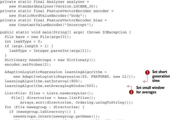
This program starts with the allocation and configuration of the learning algorithm. Here we chose AdaptiveLogisticRegression for simplicity because it isn’t necessary to worry much about its learning parameters. You might also use a CrossFoldLearner if you don’t mind tweaking learning parameters. The code configures the generation time for the underlying evolutionary algorithm
to be fairly short because the data set is relatively small and the algorithm will learn quickly ![]() . Similarly, we set the averaging window for diagnostics to be relatively short so that we get quick indications of how the
learning algorithm is doing
. Similarly, we set the averaging window for diagnostics to be relatively short so that we get quick indications of how the
learning algorithm is doing ![]() .
.
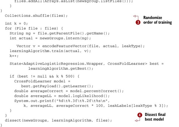
In preparation for training, we need a list of all documents in the training set. We also want to order them randomly to help
the algorithm learn more effectively. In order to train the model, we iterate over the randomly ordered document list ![]() . Training involves conversion to vector form and the actual training of the model. Once the evolutionary algorithm inside
the AdaptiveLogisticRegression gets going, it will provide the best-known model from its pool. We can use this model to get the log likelihood and percent
correct averaged over recent training examples.
. Training involves conversion to vector form and the actual training of the model. Once the evolutionary algorithm inside
the AdaptiveLogisticRegression gets going, it will provide the best-known model from its pool. We can use this model to get the log likelihood and percent
correct averaged over recent training examples.
When we complete training, we dissect the model ![]() . The details of this dissection are shown in the following listing.
. The details of this dissection are shown in the following listing.
Listing 15.4. Model dissection for 20 newsgroups example

In dissecting the model, we need to first make sure that the model’s parameters have been finalized ![]() . Closing an online model doesn’t prevent further training, but it does make sure that we have a consistent state to dissect.
. Closing an online model doesn’t prevent further training, but it does make sure that we have a consistent state to dissect.
In dissection, we need to provide the feature encoding with a so-called trace dictionary ![]() . This records which predictor variables and values were assigned to which locations in the feature vector. This slows down
the encoding by quite a bit, so it isn’t something to be done normally. By clearing the trace dictionary on each example,
or every few examples, we can avoid letting the trace dictionary grow too large in memory
. This records which predictor variables and values were assigned to which locations in the feature vector. This slows down
the encoding by quite a bit, so it isn’t something to be done normally. By clearing the trace dictionary on each example,
or every few examples, we can avoid letting the trace dictionary grow too large in memory ![]() . After encoding each example and recording the details of the feature extraction, we pass the details to the model dissector.
. After encoding each example and recording the details of the feature extraction, we pass the details to the model dissector.
Once you’ve finished processing a reasonable number of training examples, you can ask the model dissector for a list of the most important variables and values. In this example, the top 100 such values are printed.
If you run this example, you’ll see the percent correct evolve something like what is shown in figure 15.1.
Figure 15.1. Increase in average percent correct with increasing number of training examples. The gray bar shows the reasonable maximum performance level that you can expect, based on the best results reported in the research literature.

If you used multiple passes through the data used to create figure 15.1, the actual performance would likely approach state of the art performance in the mid 80 percent range. Making multiple passes doesn’t improve the model as much as training on additional previously unseen data, because repeating the same data doesn’t give as much diversity in training data. Happily, having too small a sample size is almost never the issue with Mahout-based classification, because Mahout’s claim to fame is large data sets. Multiple passes through the data do still improve the model’s performance because the system learns with every pass, up to a point.
Here is the output of the model dissection for a typical run such as shown in figure 15.1. The columns are the name of the feature (a single word of text, in this case), the largest weight of that feature, and the target variable value for that largest weight.
body=space       2.1   sci.space
body=sale        1.9   misc.forsale
body=car         1.9   rec.autos
body=windows     1.8   comp.os.ms-windows.misc
body=mac         1.7   comp.sys.mac.hardware
body=bike        1.7   rec.motorcycles
body=apple       1.5   comp.sys.mac.hardware
body=gun         1.5   talk.politics.guns
body=baseball    1.5   rec.sport.baseball
body=graphics    1.5   comp.graphics
body=key         1.5   sci.crypt
body=x           1.4   comp.windows.x
body=dod         1.4   rec.motorcycles
body=orbit       1.4   sci.space
body=clipper     1.4   sci.crypt
body=encryption  1.3   sci.crypt
body=window      1.3   comp.windows.x
body=image       1.2   comp.graphics
body=hockey      1.2   rec.sport.hockey
body=atheists    1.2   alt.atheism
These features are clearly pretty reasonable, with the possible exception of the word dod. This is apparently a feature for the rec.motorcycles Usenet discussion group. Examination of the training texts, interestingly, shows that there was a lengthy discussion back and forth using dod as a nonsense word. Although this feature is probably not going to help future performance after the presumably short-lived use of that word, it also isn’t likely to hurt.
At this point, you know how to measure how good your classifier is. That leaves you with the problem of trying to decide what those measurements mean. Let’s look at how typical problems show up in the performance metrics, and how you can diagnose and fix these problems.
15.3. When classifiers go bad
When working with real data and real classifiers it’s almost a rule that the first attempts to build models will fail, occasionally spectacularly. Unlike normal software engineering, the failures of models aren’t usually as dramatic as a null pointer dereference or out-of-memory exception. Instead, a failing model can appear to produce miraculously accurate results. Such a model can also produce results so wrong that it seems the model is trying to be incorrect. It’s important to be somewhat dubious of extremely good or bad results, especially if they occur early in a model’s development.
This section will help you understand how the metrics you collect, using techniques from the previous section, can tell you about these predictable bumps in the life of a classifier. To do that, you need to know what the common problems with classifiers are and how those problems show up in the performance metrics.
The two most common problems in building classification models are so-called target leaks and broken feature extraction. A target leak occurs when some feature in the training data provides information about the target variable in some way that won’t happen in production. This is the classifier equivalent of handing out the answers to an exam along with the exam itself. Not surprisingly, a classifier can do quite well in such a case. This sort of problem can happen in subtle ways that are difficult to diagnose. Bad feature extraction can also be difficult to detect unless it’s catastrophically bad. You’ll see examples of both problems in the next sections.
15.3.1. Target leaks
A target leak is a bug that results from information from the target variable being included in the predictor variables used to train a classifier. The major symptom of a target leak is performance that’s just too good to be true.
To help you understand how to avoid a target leak, we intentionally insert one in the 20 newsgroups sample classifier from listing 15.3. Here is the small addition to the program that injects a target leak into the training examples:
private static final SimpleDateFormat("MMM-yyyy");
// 1997-01-15 00:01:00 GMT
private static final long DATE_REFERENCE = 853286460;

...
  long date = (long) (1000 *
      (DATE_REFERENCE + target * MONTH + 1 * WEEK * rand.nextDouble()));
  Reader dateString = new StringReader(df.format(new Date(date)));
  countWords(analyzer, words, dateString);
Unlike before, this code injects a simulated target leak into the data in the form of a date field. This date field is chosen so that all the documents from the same newsgroup appear to have come from the same month, but documents from different newsgroups come from different months. Dates, times, and ID numbers are common sources of target leaks, but we could have used any sort of field to inject the leak. Even the target variable itself can accidentally be included as a predictor. As you might expect, such an error creates the mother of all target leaks.
When you train the model using this target leak in addition to the text, the accuracy of the model gets entirely too good. Figure 15.2 shows what happens. Especially in the case where the target leak appears with just the subject line, accuracy approaches 100 percent. This is unrealistically high, because the best reported result for this data set in the research literature is about 86 percent. In the case where the leak is added to all of the text from the subject line and the body of the message, it takes longer for the learning algorithm to sort out what is happening, but before long it still reaches implausibly good performance.
Figure 15.2. A target leak produces implausible accuracy, but not always instantly.

From the results shown in figure 15.2, you can see that the two lines representing conditions with the target leak quickly approach 100 percent accuracy. Such an extreme level of accuracy isn’t plausible for this problem. The SGD model without the leak, on the other hand, only just reaches the level represented by the best academic research results for this problem. That level of performance is very good, but still plausible.
When working with real data rather than carefully studied research data, it isn’t necessarily possible to known how good “too good” is from the start. If the model appears to be doing exceptionally well, or if the performance on new data is dramatically worse than predicted by cross validation, it’s worth looking at the output of the ModelDissector.
Here are the first few lines of the model dissection output from one of the cases with a target leak. The columns in the output are the term, the weight, and the newsgroup that the weight applies to.
body=feb-1998          3.7    sci.electronics
body=dec-1997          3.6    comp.graphics
body=sep-1997          3.5    sci.med
body=mar-1998          3.3    comp.sys.mac.hardware
body=jul-1997          3.3    talk.religion.misc
body=jun-1997          3.2    misc.forsale
body=apr-1998          3.2    rec.motorcycles
body=jul-1998          3.1    talk.politics.misc
body=jun-1998          3.0    comp.os.ms-windows.misc
body=mar-1997          2.9    sci.space
body=apr-1997          2.9    talk.politics.guns
body=jan-1998          2.8    soc.religion.christian
body=nov-1997          2.8    comp.sys.ibm.pc.hardware
body=may-1997          2.8    comp.windows.x
body=feb-1997          2.7    rec.sport.baseball
body=aug-1998          2.6    alt.atheism
body=may-1998          2.6    rec.autos
body=oct-1997          2.5    rec.sport.hockey
body=gun               2.1    talk.politics.guns
body=aug-1997          2.1    sci.crypt
body=windows           2.0    comp.os.ms-windows.misc
body=consciously       1.8    sci.electronics
body=taber             1.8    sci.electronics
body=uw.pc.general     1.8    sci.electronics
body=hearing           1.8    sci.med
body=car               1.7    rec.autos
[email protected]   1.7    misc.forsale
body=1024x768x24       1.7    comp.graphics
body=contradicts       1.7    talk.religion.misc
body=market            1.7    comp.graphics
body=passes            1.7    misc.forsale
body=att-14,796        1.7    talk.religion.misc
body=bars              1.7    sci.med
These most heavily weighted features are dominated by dates. Other than large-scale seasonal changes, like Christmas, having the date be such a strong predictor of topic isn’t reasonable. Having nearly all of the top 20 features be particular dates is entirely too much to believe, so the only reasonable conclusion is that these features represent a target leak. Of course, in this case, we intentionally injected the target leak, so nobody should be surprised to find one.
Another, more subtle, indicator that something is wrong comes from looking at the top nonleak features. The AdaptiveLogisticRegression adjusts the learning rate in order to optimize performance. In the case of a target leak, it’s to the advantage of the algorithm to decrease the training rate fairly quickly once it has found the leak features. As such, it can freeze other extraneous features without their weights decaying to 0, as a normal model would have to do to get good performance. As a result, you’ll see words like taber, market, passes, and bars listed as highly weighted features, predictive of sci.electronics, comp.graphics, misc.forsale, and sci.med respectively. That such features persist in the final model is an indication that learning has frozen without proper pruning.
15.3.2. Broken feature extraction
Another common problem occurs when the feature extraction is somehow broken. In contrast to target leaks, where performance is unreasonably good, broken feature extraction causes much worse performance than expected.
The following code shows how a Lucene tokenizer should be used for the tokenization of the 20 newsgroups data.
TokenStream ts = analyzer.tokenStream("text", in);
ts.addAttribute(TermAttribute.class);
while (ts.incrementToken()) {
  String s = ts.getAttribute(TermAttribute.class).term();
  words.add(s);
}
An easy error to make would be to try to get the text token by using s = ts .toString() instead of using the correct, but slightly obscure, call to term(). Committing this error in tokenization causes additional information to be retained in addition to the desired token, and this additional information makes the same word in different locations appear as if it were two different words. That makes learning from the affected predictor hard, if not impossible.
Figure 15.3 shows what performance looks like with the tokenization error in place. The percent correct never gets much above 5 percent, which is, of course, the result the model would get by randomly selecting a result.
Figure 15.3. Performance with the tokenization bug never increases above the level expected from a random selection of the target variable. The gray line shows the performance that would be expected by chance.

This example is extreme because all the input data has been corrupted by bad tokenization; nothing is left that the model can use to produce good results. In practice, it’s more common that only some fields are corrupted and others are fine. Such a partial corruption will lead to degraded performance if the corrupted variable would have helped the model, but it won’t necessarily lead to the flat-line performance that you see in this example because the uncorrupted variables are still available to carry some of the load.
The best way to find these kinds of problems is to compute summary statistics on the values being encoded. If the value is continuous, use an OnlineSummarizer to examine the mean, minimum, maximum, and quartiles. These values should seem reasonable. For categorical, word-like, and text-like data, you should produce counts of the tokens produced and plot these counts versus rank on a log-log scale. For the 20 newsgroups data, this gives a graph like the one shown in figure 15.4. For word-like and text-like data, something similar should emerge for each field of your data. In the case of our injected tokenization error, the frequencies of essentially all terms would be exactly 1.
Figure 15.4. Plot of token count versus rank for a correctly operating tokenizer on the 20 newsgroups data. With the broken tokenizer, the counts would all have a value of 1.

Table 15.4 shows some of the incorrect tokens that are produced if insertTokenError is set along with the correct values that should have been produced. Keep in mind that the parentheses, commas, and numbers are all part of the incorrect tokens.
Table 15.4. How bad tokens can defeat feature extraction
|
Erroneous token |
Correct token |
|---|---|
| (term=elastic,startOffset=1705,endOffset=1712,...) | elastic |
| (term=elastic,startOffset=2064,endOffset=2071,...) | elastic |
| (term=failed,startOffset=1236,endOffset=1242,...) | failed |
| (term=failed,startOffset=245,endOffset=251,...) | failed |
| (term=failed,startOffset=974,endOffset=980,...) | failed |
Note how repeated instances of the same token in the table appear different if too much information is inadvertently retained. This situation makes these erroneous tokens useless for categorization because the chances that they’ll appear in another document at exactly the same place are nearly nil.
Now that you know how some pitfalls such as target leaks and broken feature extraction can defeat a classifier, let’s turn to a more optimistic topic and see how you can use evaluation to adjust and tune a classifier to improve performance.
15.4. Tuning for better performance
Beyond correcting errors in training data, you can do a lot to improve classifier performance. Some approaches involve making the classifier’s life easier by changing the problem itself. Others involve making the classifier run better on the data given. In the first case, it’s possible to find new predictor variables, combinations of predictors, or transformations of predictors to help the classifier out. It’s also possible to eliminate predictors that aren’t helping or to simplify the target variable. In the second case, learning rates can be tuned or feature encoding strategies adjusted in the learning algorithm.
In any case, when tuning a classifier system, you need to make careful and realistic measurements of performance with and without the changes. It isn’t usually sufficient to examine a few ad hoc examples unless your change has made a dramatic difference. In fact, once the system is working reasonably, most adjustments should improve or degrade performance by only small amounts, which can only be detected with accurate measurement.
15.4.1. Tuning the problem
To most people, the idea of tuning up a classification system brings to mind the idea of tuning the learning algorithm so that its accuracy is as high as possible. This assumption leads to trouble, however, because it misses some of the best opportunities. Often the big improvements result from tuning the problem instead. This approach can include changing the input, the output, or even the interpretation of the output.
Remove Fluff Variables
Some variables don’t help the classifier much or even at all, and it may be better to simply withhold these variables from the classifier. Paradoxically, removing some information like this can improve accuracy because the learning algorithm may have less distraction with fewer variables and thus may learn a better classifier in the available training time. The target leak problem shown in section 15.4 was a great example of this phenomenon. In that example, the learning algorithm took considerably more time to learn the trivial target leak model when it had lots of text around to distract it. Conversely, you could say that the leak variable itself distracted the learning algorithm and prevented it from noticing the really helpful variables in the subject or body.
Regularization is a more general version of this idea. Regularization is a mathematical technique that’s used to avoid over-fitting by decreasing the effect of some variables or even eliminating them entirely. Regularization operates by having the learning algorithm learn to minimize error and model complexity at the same time. The mathematical function that penalizes complexity is called the prior in Mahout terminology.
Algorithms such as SGD with regularization try to eliminate variables, where possible, by penalizing the inclusion of variables in the model. All else equal, these algorithms would prefer to not include a variable. Even so, it can take time for these algorithms to understand which variables can be eliminated. If dissecting a model shows that some variables are never mentioned in the model, it’s probably useful to try eliminating them so that subsequent training goes faster. Likewise, it’s useful to test versions of the model that aren’t allowed to use certain categories of variables, to see what happens.
Other Mahout classifier algorithms, like naive Bayes and complementary naive Bayes, can benefit greatly from the elimination of variables that don’t carry useful information, because these algorithms have no mechanism to eliminate these variables on their own via regularization.
It’s relatively common to find that removing one of two variables makes no difference, but removing both seriously hurts performance. It can also happen that using a particular variable alone gives no better performance than chance decisions. It would be tempting to eliminate that variable if you noticed this lack of performance. Occasionally, however, such a variable would be able to improve the performance of other variables, even though it shows no predictive qualities in isolation. It’s safe to say that any variable that doesn’t appear in the dissection of the final model can be eliminated with positive effect, but most other conclusions require careful testing.
Add New Variables, Interactions, and Derived Values
In building a classification system, some data is easier to wrangle into usable form than other data. Difficulties in data preparation will usually lead to delays in being able to present all of the desired predictor variables to the learning algorithm. Conversely, some variables will probably be available sooner than others. In a large project, the delays in getting certain predictors can easily extend to weeks or months, and some predictors may well turn out to be impossible to get.
The potential for these delays means that modeling and evaluation should be started early, with whatever data is available. It often happens that the initially available predictor variables are sufficient to build a deployable model. Additional variables should be tested as they become available, because they may improve performance even if the early models are usable in production.
Another common source of new variables is the transformation of existing continuous variables. It can pay to insert additional versions that are the logarithm or the square of the original value. Generalized linear models, such as the Mahout SGD-based models, can benefit from this technique, because they otherwise notice only linear relationships between predictors and categories. Most tree-based models won’t notice the difference.
Here’s an example where a TrainingExample object is queried for a line count that’s then encoded three different ways:

By encoding the line count transformed in multiple ways, we’ve provided the model with the ability to make certain kinds of inferences much more easily. For example, including logs of original and sale prices gives the model access to the equivalent of a discount percentage. Giving it only the original and sale prices untransformed allows it to only see discounts in dollar terms rather than as a fraction of the original price. Which view is better is hard to say in advance, so letting the learning algorithm choose can be a very good idea.
It doesn’t make sense to add multiple versions of a variable for a naive Bayes model because naive Bayes only accepts categorical or text-like inputs. These inputs are encoded as a number of binary values, and transformations of binary variables rarely make any useful sense.
Interaction variables are combinations of other variables, and they’re another source of power for a classifier. For instance, in a marketing application, it might be very good to have an interaction variable that combines gender with brand name. Without this interaction variable, the model can deduce that women are more or less likely to respond to a marketing offer than men, or that a particular brand is more or less popular. With the interaction of gender and brand, however, the model can say that a particular brand is more or less popular with men or more or less popular with women. Because different manufacturers specialize the brands they sell to appeal to different market segments, it’s no surprise that such a variable can be very useful. With hashed feature representations, interaction variables can be added using code similar to the following:
LuceneTextValueEncoder authorEnc = new LuceneTextValueEncoder("author");
LuceneTextValueEncoder subjectEnc = new LuceneTextValueEncoder("subject");
FeatureVectorEncoder authorPlusSubjectEnc =
      new InteractionValueEncoder("author_subject", author, subject);

for (TrainingExample example : trainingData) {
  Vector v = new RandomAccessSparseVector(50000);
  String author = example.getAuthor();
  String subject = example.getSubject();
  authorEnc.addToVector(author, 1, v);
  subjectEnc.addToVector(subject, 1, v);
  authorPlusSubjectEnc.addToVector(author, subject, 1, v);
  ...
}
Here, the authorPlusSubjectEnc interaction encoder is created using a reference to the authorEnc author encoder and the subjectEnc subject text encoder. The string containing the author name and subject line is encoded by encoding author, subject, and the combination as an interaction variable. The interaction variable represents not just the author and subject, but the fact of their association, distinct from that subject as used by another author or that author talking about a different subject. This allows the classifier to draw different distinctions based on both who and what was said. If different authors use the same text to mean different things, the model would have no chance of learning the correct meaning without this interaction variable. But with it, the model can ascribe different meanings to exactly the same words, depending on the context in which they appear. In addition, because of the inclusion of the separate encoders for author and subject, the model can also learn subject line meanings that don’t depend on who authored the subject line.
Interactions are powerful, but they can dramatically increase the complexity of a classifier and make feature encoding and learning dramatically slower. Because the number of features for each training example is dramatically increased, this can also cause accuracy to degrade.
Another way to introduce transformations of existing variables is to cluster a portion of training data, applying something like k-means clustering to several of the predictor variables. This clustering leads to a new predictor: for each piece of data, its cluster is a categorical feature.
Similarly, it’s possible to build a classifier model and then use the output of that classifier as a predictor variable for another model. The idea is that the first model will learn the general outline of the problem, and the cascaded second model can learn how to correct errors that the first model makes. Here is a bit of code that illustrates this:
AbstractVectorClassifier subModel =
    ModelSerializer.readBinary(new FileReader("sub-model.model"),
    OnlineLogisticRegression.class);
ConstantValueEncoder subModelEnc = new ConstantValueEncoder("sub");
...
for (TrainingExample example : trainingData) {
  Vector v1 = new RandomAccessSparseVector(50000);
  ... encode features for subModel ...
  Vector v2 = new RandomAccessSparseVector(50000);
  double subScore = subModel.classifyScalar(v1);
  subModelEnc((byte[]) null, subScore, v2);
  ... encode other features ...
  ... train model ...
}
Here we assume that there’s a first model already trained and available in the file submodel.model. Then when training the second model, we build a feature vector to be used as input for the first model, and run that first model to compute a score. That score is then used as a feature for the second model.
15.4.2. Tuning the classifier
In addition to changing the data that’s presented to the classifier learning algorithm, it’s possible to change the algorithm or to modify the parameters that define the algorithm. The benefit of trying these approaches is that it provides you with a variety of ways to improve performance through guided trial and error.
Try Alternative Algorithms
It’s important to test different classifier algorithms to see which algorithm does best. Mahout supports naive Bayes, complementary naive Bayes, and SGD. There are also experimental implementations of random forests and support vector machine (SVM) available.
In addition to changing the entire class of model, it’s possible to change the learning algorithm while keeping the same kind of model. In particular, SGD-based classifiers can operate the low-level learning algorithm with cross validation using CrossFoldLearner, or the self-adapting AdaptiveLogisticRegression, which adjusts the many learning parameters automatically. There’s also the choice of just what the learning algorithm is optimizing, choosing from log likelihood, AUC, or mixtures of these.
Compare different algorithms based on performance, training time, and classification speed. For example, try both versions of the Bayes algorithms as well as AdaptiveLogisticRegression. If more than one model does reasonably well on accuracy metrics, decide between them based on how well they integrate with the rest of the system.
Tune the Learning Algorithm
Particularly with the low-level SGD learning algorithms, there are many knobs that can be turned to get different results. Most of these parameters are adjusted when constructing an AdaptiveLogisticRegression, CrossFoldLearner, or OnlineLogisticRegression using similar configuration methods. These methods are summarized in table 15.5.
Table 15.5. Configuration methods for SGD learning classes
|
Algorithm parameter |
How configured |
Online logistic regression |
Cross fold learner |
Adaptive logistic regression |
Description |
|---|---|---|---|---|---|
| prior | Constructor | Yes | Yes | Yes | Sets the regularization function to encourage sparsity and avoid overfitting |
| numFeatures | Constructor | Yes | Yes | Yes | Specifies the size of the feature vector |
| numCategories | Constructor | Yes | Yes | Yes | Specifies how many target categories there are |
| alpha | Setter | Yes | Yes | Sets learning rate schedule | |
| decayExponent | Setter | Yes | Yes | Sets learning rate schedule | |
| lambda | Setter | Yes | Yes | Controls amount of regularization | |
| learningRate | Setter | Yes | Yes | Sets learning rate schedule | |
| stepOffset | Setter | Yes | Yes | Sets learning rate schedule |
The prior, number of features, and number of target categories are configured in all SGD classes in the constructor. The AdaptiveLogisticRegression class controls the learning rate by running a number of CrossFoldLearners in parallel with different settings, and comparing the results obtained with each of them. This means that with AdaptiveLogisticRegression, the only other configuration settings needed are those used to control how often the learning rate is changed and how many different parallel CrossFoldLearners are used to test different settings. For the CrossFoldLearner and OnlineLogisticRegression, you need to specify the learning rate and also how the learning rate will decay over time. This is done using builder-style methods such as those shown here:
lr = new CrossFoldLearner(targetCategories, numFeatures, new L1())
          .lambda(currentLambda)
          .learningRate(initialLearningRate)
          .decayExponent(0.5)
          .stepOffset(2000);
Usually, decayExponent and stepOffset are used to control how the initial learning rate is decreased over time; setting alpha is much less common.
In addition to these settings, the CrossFoldLearner allows you to set the number of cross-validation folds it uses internally. The default value of 5 is acceptable in almost all cases. Using a lower value, such as 2 or 3, decreases the amount of data available for training more than most applications are willing to accept, and setting the value much higher than 5 incurs higher computation costs because it needs an independent learner for each fold.
The simplest approach to tuning all of these parameters is to just use AdaptiveLogisticRegression with the default settings. But this costs quite a bit in terms of computing power, because the AdaptiveLogisticRegression uses an internal evolutionary pool of 20 CrossFoldLearners, each of which internally maintains 5 OnlineLogisticRegression objects. This means you pay the cost of running 100 learning algorithms at the same time.
In practice, though, the penalty is much smaller than that because reading training examples from disk and encoding them as feature vectors often costs nearly as much as running the 100 learning algorithms. Moreover, in practical situations, a learning algorithm will be run with at least dozens and possibly hundreds or thousands of settings for these parameters. The AdaptiveLogisticRegression does all that automatically. As a side effect, data must only be encoded once. Bad options are cut off early, so no computational power is wasted on them.
15.5. Summary
You’ve now seen the major APIs in Mahout for computing classification quality metrics, and you’ve seen the basics of how to use these metrics. You know how common bugs affect these metrics and how to find and correct common problems with classification.
As the examples in this chapter have shown, problems with classifiers can be subtle. Unlike in most computer programming, even a serious error may not cause complete failure because learning algorithms often learn how to compensate for partial failures. This situation is both good and bad news, and it makes detailed quality testing important.
Evaluation isn’t only an iterative process during the steps of building and tuning a high-performing classifier; it’s also an important ongoing step after production launches. Evaluating performance over time is critical to maintaining performance. External conditions may change, making the model less useful, or operational errors in data collection can degrade a model’s effectiveness. In any case, ongoing evaluation during production is key to being able to recognize the need to retune or retrain a model or opt for a new approach. These issues are explored in the discussion of deployment in the next chapter.