Chapter 14. Training a classifier

This chapter covers

• Extracting features from text
• Converting features for Mahout’s use
• Training two Mahout classifiers
• Selecting from among Mahout’s learning algorithms

This chapter explores the first stage in classification: training the model. Developing a classifier is a dynamic process that requires you to think creatively about the best way to describe the features of your data and to consider how they will be used by the learning algorithm you choose to train your models. Some kinds of data lend themselves readily to classification; others offer a greater challenge, which can be rewarding, frustrating, and interesting all at once.

In this chapter, you’ll learn how to choose and extract features effectively to build a Mahout classifier. Feature extraction involves much more than the simplified steps you saw in the examples in chapter 13. Here we go into the details of feature extraction, including how to preprocess raw data into classifiable data and how to convert classifiable data into vectors that can be used by the Mahout classification algorithms. We use a computational marketing problem as an example to show how training data might be extracted from a database.

Once you understand how to get data ready for classification, in section 14.4 you’ll build a classifier using a standard data set—20 newsgroups—with the Mahout algorithm known as stochastic gradient descent (SGD).

In section 14.5, we review the characteristics of the various learning algorithms available for use with Mahout classification and help you decide how to choose the ones best suited to particular projects. These two steps, extracting features and choosing the algorithm, go hand in hand in designing and training a classifier, and to help you develop an intuitive sense of the different options, we look at a second step-by-step example using a different learning algorithm, naive Bayes, with the same 20 newsgroups data set.

This chapter starts by explaining how to work with the data in your training examples.

14.1. Extracting features to build a Mahout classifier

Getting data into a form usable by a classifier is a complex and often time-consuming step, and in this section we present an overview of what is involved. You saw a simplified view of the training and use of a classification model in figure 13.2 (in chapter 13); it showed a single step leading from training examples to the training algorithm that trains the classification model. But in reality, the situation is more complex. The important details not mentioned in chapter 13 are shown here, in figure 14.1.

Figure 14.1. An expansion of part of figure 13.2 from the previous chapter. This is what must be done to get raw data ready so that it can be input into a training algorithm.

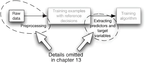
Figure 13.2 showed a single step leading from the training data to the training algorithm. In reality, raw data must be collected and preprocessed to turn it into classifiable training data. The training examples in figure 14.1 are classifiable data—we’ll cover the processing of raw data into classifiable data in this chapter and in more detail in chapters 15 and 16.

Once the raw data has been preprocessed into classifiable form, several steps are required to select predictor and target variables and encode them as vectors, the style of input required by Mahout classifiers. Recall from chapter 13 that the values for features to be used as predictor variables can be of four types:

• Continuous
• Categorical
• Word-like
• Text-like

This description of predictor variables is correct on the whole, but it omits the important fact that when the values are presented to any of the algorithms used to train a classifier, they must be in the form of vectors of numbers, either in memory or in a file format that the training algorithm can read.

Compare the simplified sequence depicted in figure 14.1 with the more detailed diagram in figure 14.2. The original data undergoes changes in order to turn it into the vectors required as input for the training algorithm. These changes happen in two phases: preprocessing, to produce classifiable data for use as training examples, and converting classifiable data into vectors.

Figure 14.2. Vectors are the format that the classification algorithms require as input. In order to encode data as vectors, raw data must be collected in a single record in classifiable format, ready for parsing and vectorization.

As figure 14.2 shows, preparing data for the training algorithm consists of two main steps:

1. Preprocessing raw data—Raw data is rearranged into records with identical fields. These fields can be of four types: continuous, categorical, word-like, or text-like in order to be classifiable.
2. Converting data to vectors—Classifiable data is parsed and vectorized using custom code or tools such as Lucene analyzers and Mahout vector encoders. Some Mahout classifiers also include vectorization code.

The second of these steps has two phases: tokenization and vectorization. For continuous variables, the parsing may be trivial, but for other types of variables, such as categorical, word-like, or text-like variables, vectorization can be involved.

We’ll discuss these two steps in detail in subsequent sections of this chapter.

14.2. Preprocessing raw data into classifiable data

The first phase of feature extraction involves rethinking the data and identifying features you could use as predictor variables. You first select a target variable that’s in accordance with the goal of classification and pick or drop features to get a mix that’s worthy of an initial try. There is no exact recipe: this step calls for intelligent guessing guided by experience, and as you work through the examples in this chapter, you’ll be on your way toward getting that experience.

This section offers a brief overview of how to preprocess data. The steps include collecting or rearranging data into a single record, and gleaning secondary meanings from raw data (such as converting a ZIP code to a three-digit code or using a birth date to determine age). Preprocessing isn’t a prominent part of the examples in this chapter, because this phase of data extraction has essentially already been done for you in the data set you’ll be using here. Preprocessing plays a larger role in the examples in chapters 16 and 17.

14.2.1. Transforming raw data

Once you identify the features you want to try out, they must be converted into a format that’s classifiable. This involves rearranging the data into a single location and transforming it into an appropriate and consistent form.

Note

Classifiable data consists of records with identical fields that contain one of four types of data: continuous, categorical, word-like, or text-like. Each record contains the fully denormalized description of one training example.

At first glance, it may seem like this step is already done: if the data looks like words, it must be words, right? If the data looks like numbers, it must be continuous, yes? But as you saw in chapter 13, first appearances can be a little misleading. For example, a ZIP code looks like a number but it’s actually a category, a label for predetermined classes. Things that contain words may be word-like, or they may best be considered as categories or text. ID codes for users or products may look like numbers, categorical, or word-like data, but more commonly, they should be denormalized away in favor of the characteristics of the user or product that they link to.

The following example from computational marketing provides an exercise in preparing raw data for use in classification.

14.2.2. Computational marketing example

Suppose you’re trying to build a classification model that will determine whether a user will buy a particular product if they’re offered it. This isn’t quite a recommendation system because it’ll classify examples by using user and product characteristics rather than the collective behavior of similar users.

For this example, you have a database with several tables in it, as shown in figure 14.3. The tables are typical of a highly simplified retail system. There are tables representing users and products, a table recording when products were offered or shown to users, and a table that records purchases that arise from showing a product to a user. This data isn’t currently acceptable as training or test data for a classifier because it’s spread across several tables.

Figure 14.3. Table structure for a product sales example containing different types of data. Because no record in any table contains the data necessary in a training example for a classifier, this organization of raw data isn’t directly usable as training data.

The marketing project depicted in figure 14.3 has a wide variety of data types. Users have demographic data, such as birth date and gender; products have type and color. Offers of products to users are recorded in the offer table, and purchases of products subsequent to an offer are recorded in the purchase table.

Figure 14.4 shows how this data might become training data for a classifier. There would be one of these records for each record in the offer table, but note how user and product IDs have been used to join against the user and product tables. In the process, the user’s birth date is expressed as an age. An outer join has been used to derive the delay between offer and purchase as well as to add a flag indicating whether a purchase was ever made.

Figure 14.4. To get classifiable data, training examples are constructed from several sources to denormalize everything into a single record that describes what happened. Some variables are transformed; birth date is expressed as an age, and purchase time is expressed as a delay.

In order to get the data represented in the tables into the usable form shown in figure 14.4, it needs to be brought together and rearranged. To do this, you might use an SQL query like this:

select
  now()-birthDate as age, gender,
  typeId, colorId, price, discount, offerTime,
  ifnull(purchase.time, 0, purchase.time - offer.time) as purchaseDelay,
  ifnull(purchase.time, 0, 1) as purchased
from
  offer
  join user using (userId)
  join product using (productId)
  left outer join purchase using (offerId);

This query denormalizes the data stored in the separate database tables into records that contain all the necessary data. The driving table here is the offer table, and the nature of the foreign keys for userId, productId, and offerId force the output of this query to have exactly one record for each record in the original offer table. Note how the join against the purchase table is an outer join. This allows the ifnull expressions involving purchase.time to produce 0s if there is never a purchase.

Note

Sometimes age is better for classification, and sometimes birth date is better. For instance, in the case of insurance data on car accidents, age will be a better variable to use because having car accidents is more related to life-stage than it is to the generation a person belongs to. On the other hand, in the case of music purchases, birth date might be more interesting because people often retain early music preferences as they get older. Their tastes often reflect those of their generation.

The records that come out of this query are now in the form of classifiable data, ready to be parsed and vectorized by the training algorithm. The next steps can be done using code you write or by putting the data into a format accepted by Mahout classifiers (which contain their own parsing and vectorization code). The following section and examples focus on vectorizing the parsed, classifiable data.

14.3. Converting classifiable data into vectors

In Mahout parlance, a Vector is a data type that stores floating-point numbers indexed by integers. This section of the chapter will show you how to encode data as Vectors, explain what feature hashing is, and demonstrate how the Mahout API does feature hashing. We also look at how you can encode the different types of values associated with variables.

You saw Vectors used previously in the chapters on clustering. Many kinds of classifiers, especially ones available in Mahout, are fundamentally based on linear algebra and therefore require training data to be input in the form of Vectors.

14.3.1. Representing data as a vector

How do you represent classifiable data as a Vector? There are several ways to do this, and they’re summarized in table 14.1.

Table 14.1. Approaches to encoding classifiable data as a vector

Approach	Benefit	Cost	Where used?
Use one Vector cell per word, category, or continuous value	Involves no collisions and can be reversed easily	Requires two passes (one to assign cells and one to set values) and vectors may have different lengths	When dumping a Lucene index as Vectors for clustering
Represent Vectors implicitly as bags of words	Involves one pass and no collisions	Makes it difficult to use linear algebra primitives, difficult to represent continuous values, and you must format data in a special non-vector format	In naive Bayes
Use feature hashing	Involves one pass, vector size is fixed in advance, and it’s a good fit for linear algebra primitives	Involves feature collisions, and the interpretation of the resulting model may be tricky	In OnlineLogisticRegression and other SGD learners

The approaches listed in table 14.1 are used in different classifiers in Mahout. Let’s begin by looking at how to encode word-like, text-like, and categorical values as Vectors.

One Cell Per Word

One way to encode classifiable data as a Vector involves making two passes through the training data: one to determine the necessary size of the Vector and build a dictionary that remembers where every feature should go in the Vector, and then another to convert the data. This approach can use a simple representation for encoding training and test examples: every continuous value and every unique word or category in categorical, text-like, and word-like data is assigned a unique location in the vector representation.

The obvious downside to this approach is that passing through the training data twice has the potential for making the training of the classifier twice as computationally expensive, which can be a real problem with very large data sets.

This two-pass approach is used by most of the clustering algorithms in Mahout.

Vectors as Bags of Words

Another approach is to carry around the feature names or names plus category, word, or text values instead of carrying around a Vector object. This method is used primarily by Mahout classifiers like naive Bayes and complementary naive Bayes.

The advantage of this approach is that it avoids the need for a dictionary, but it means that it’s difficult to make use of Mahout’s linear algebra capabilities that require known and consistent lengths for the Vector objects involved.

Feature Hashing

SGD-based classifiers avoid the need to predetermine vector size by simply picking a reasonable size and shoehorning the training data into vectors of that size. This approach is known as feature hashing. The shoehorning is done by picking one or more locations by using a hash of the name of the variable for continuous variables, or a hash of the variable name and the category name or word for categorical, text-like, or word-like data.

This hashed feature approach has the distinct advantage of requiring less memory and one less pass through the training data, but it can make it much harder to reverse-engineer vectors to determine which original feature mapped to a vector location. This is because multiple features may hash to the same location. With large vectors or with multiple locations per feature, this isn’t a problem for accuracy, but it can make it hard to understand what a classifier is doing.

14.3.2. Feature hashing with Mahout APIs

In this section, we look at how to do feature hashing using the Mahout API. We present in detail how to encode continuous, categorical, word-like, and text-like features. We also explain what feature collisions are and how they may affect your classifier.

Encoding Continuous Features

Continuous values are the easiest kind of data to encode. The value of a continuous variable gets added directly to one or more locations that are allocated for the storage of the value. The location or locations are determined by the name of the feature.

Mahout supports hashed feature encoding of continuous values through ContinuousValueEncoder. By default, the ContinuousValueEncoder only updates one location in the vector, but you can specify how many locations are to be updated by using its setProbes() method. To encode a value for one variable, a Vector is needed: new RandomAccessSparseVector(lmp.getNumFeatures()). The value is then encoded with encoder.addToVector(value, vector). Note that the value being encoded is assumed to be a string. If the value being encoded is available as a double, then pass a null for the String value and use the weight as the value: encoder.addToVector(null, value, vector).

Encoding Categorical and Word-Like Features

Categorical features that have n distinct values can be encoded by storing the value 1 in one of n vector locations, to indicate which value the variable has. To decrease redundancy, it’s also possible to use n−1 locations and then encode the nth category by storing a 1 in no location at all (all 0s).

Hashed feature encoding is similar, but the locations are scattered throughout the feature vector using the hash of the feature name and value. In addition, each category can be associated with several locations. An additional benefit of feature hashing is that the unknown and unbounded vocabularies typical of word-like variables aren’t a problem.

To encode a categorical or word-like value using feature hashing, create a WordValueEncoder. This encoder is used in the same way the ContinuousValueEncoder was used, except that the default number of probes is two and the location being updated varies according to the value specified as well as the name of the variable. There are two kinds of this encoder: AdaptiveWordValueEncoder builds a dictionary on the fly to estimate word frequencies, so that it can apply larger weights to rare words; StaticWordValueEncoder uses a supplied dictionary or gives equal weights to all words if no dictionary is given.

Some learning algorithms are substantially helped by good word weighting, but others, like the OnlineLogisticRegression class described later, aren’t much affected by equal weights for all words.

Encoding words with equal weighting is similar to how continuous values were encoded. Here is some sample code that shows how to encode continuous variables:

FeatureVectorEncoder encoder =
    new StaticWordValueEncoder("variable-name");

for (DataRecord ex: trainingData) {
  Vector v = new RandomAccessSparseVector(10000);
  String word = ex.get("variable-name");
  encoder.addToVector(word, v);
  // use vector
}

In this code, a StaticWordValueEncoder is constructed and assigned a name that determines the seed for a random number generator. Internally, values are encoded by combining the name of the variable and the word being encoded to get locations to be modified by the encoding operation.

Sizing the vector requires experimentation. Larger vectors consume more memory and slow down the training. Smaller vectors eventually cause so many feature collisions that the learning algorithm can’t compensate.

Encoding Text-Like Features

Encoding a text-like feature is similar to encoding a word-like one except that text has many words. In fact, the example here simply adds up the vector representations for the words in the text to get a vector for the text. This approach can work reasonably well, but the more nuanced approach of counting the words first and then producing a representation that’s a weighted sum of the vectors for unique words can produce better results. This second approach is illustrated later in this chapter.

Tip

Text-like data values are ordered sequences of words, but considering the ordering of the words in text is often not necessary to get good accuracy. Simply counting the words in a text, ignoring order, is usually sufficient. That being said, the best vector for text isn’t usually just the sum of the vectors for the words in the text weighted by the counts of the words. Instead, the word vectors are usually best weighted by some function of the number of times that the corresponding word appeared in the text. Commonly used weight functions are the square root, the logarithm, or equal weighting for all words that appear, regardless of their frequency. The example in listing 14.1 uses linear weighting for simplicity, but weighting by the logarithm of the count is a better starting point for most applications.

Listing 14.1 shows how to encode text as a vector by encoding all of the words in the text independently, and then producing a linearly weighted sum of the encodings of each word. This is accomplished with a StaticWordValueEncoder and a way to break down or parse the text into words. Mahout provides the encoder and Lucene provides the parser.

Listing 14.1. Tokenizing and vectorizing text

This code produces a printable form of the vector, like this:

{8:1.0,21:1.0,67:1.0,77:1.0,87:1.0,88:1.0}

A graphical form of this output is shown in figure 14.5.

Figure 14.5. A vector that encodes text to magically vectorize. There are six nonzero values in this vector, which has a size of 100. Values equal to 0 aren’t stored and thus aren’t shown in results like these produced by the Lucene standard analyzer.

You can see in figure 14.5 that locations 8 and 21 encode the word text, locations 77 and 87 encode vectorize, and locations 67 and 88 encode magically. The word to is eliminated by the Lucene standard analyzer. The overall result of this process is a sparse vector, in which values equal to 0 aren’t stored at all.

Feature Collisions

The hashed feature representation for data can lead to collisions where different variables or words are stored in the same location. For instance, if you had used a vector with length 20 instead of the 100-long vector in the preceding example, you would have gotten the following result as the encoded value of text to magically encode:

{1:1.0,7:2.0,8:2.0,17:1.0}

In this vector, locations 7 and 8 have a value of 2 instead of 1, like all the nonzero cells in the vector shown in figure 14.5. How this happens is shown in figure 14.6.

Figure 14.6. When the vector is size 20 instead of 100, collisions occur. The terms text and magically collide at location 8, and the terms magically and vectorize collide at location 7. These collisions make it more difficult to interpret the resulting vector, but typically they don’t affect classification accuracy.

Dealing with feature collisions to avoid hurting performance can be fairly easy. In the vector shown in figure 14.6, the word text is encoded in locations 1 and 8, magically in locations 7 and 8, and vectorize in locations 7 and 17. This means that text and magically share location 8, and vectorize and magically share location 7. So locations 7 and 8 contain a value of 2, instead of 1 for all of the other nonzero values. Because each word has two locations assigned to it, the learning algorithm can learn to compensate for these collisions.

In this example, the learning algorithm can compensate for collisions because the transformation from words to vector is invertible. This would not normally be true if each word had a single location, because the vector dimension will almost always be smaller than the vocabulary of the text. With multiple locations, however, this vectorization technique usually works for the same reasons that Bloom filters work.

Where there is a collision between two words that have quite different meanings for the classifier, it’s unlikely that the other locations for these two words will also collide and it’s also unlikely that either will collide with a third word that presents the same problem. On average, therefore, this vectorization technique works well, and if the vector length chosen is large enough, there will be no measurable loss of accuracy. Exactly how long is long enough is subject to empirical validation by using the evaluation techniques you’ll see in chapter 16.

Let’s try these approaches with some real-world data using the SGD Mahout classification algorithm. (We discuss the different Mahout classification algorithms in section 14.5, and in section 14.6, you’ll have another chance to classify the same data set with a different Mahout algorithm.)

14.4. Classifying the 20 newsgroups data set with SGD

In this section, you’ll build a classification model for the 20 newsgroups data set using the learning algorithm known as SGD. In this example, you’ll preview data and do the preliminary analysis, analyze which are the most common headers, convert the data to vector form through parsing and tokenizing, and train code for the 20 newsgroups data set project.

Note

The 20 newsgroups data set is a standard data set commonly used for machine learning research. The data is from transcripts of several months of postings made in 20 Usenet newsgroups from the early 1990s.

This example emphasizes feature extraction and focuses largely on the second phase of feature extraction, vectorization. The 20 newsgroups data set is useful here because the first phase of feature extraction, preprocessing raw data into classifiable data, will be relatively simple—the researchers who created the data set have already done most of the work.

14.4.1. Getting started: previewing the data set

The first step in preparing a data set is to examine the data and decide which features might be useful in classifying examples into categories of the chosen target variable—in this case each of the 20 newsgroups.

To begin, download the 20 newsgroups data set from this URL: http://people.csail.mit.edu/jrennie/20Newsgroups/20news-bydate.tar.gz. This version of the data set splits training and test data by date and keeps all of the header lines. The date split is good because it’s more like the real world, where you’ll want to process new data with your classifier rather than old data.

If you examine one of the files in the training data directory, such as 20news-bydate-train/sci.crypt/15524, you’ll see something like this:

From: [email protected] (Ron "Asbestos" Dippold)
Subject: Re: text of White House announcement and Q&As
Originator: [email protected]
Nntp-Posting-Host: qualcom.qualcomm.com
Organization: Qualcomm, Inc., San Diego, CA
Lines: 12

[email protected] (Ted Dunning) writes:
>nobody seems to have noticed that the clipper chip *must* have been
>under development for considerably longer than the 3 months that
>clinton has been president. this is not something that choosing
...

The 20 newsgroups data set consists of messages, one per file. Each file begins with header lines that specify things such as who sent the message, how long it is, what kind of software was used, and the subject. A blank line follows, and then the message body follows as unformatted text.

The predictor features in this kind of data are either in the headers or in the message body. A natural step when first examining this kind of data is to count the number of times different header fields are used across all documents. This helps determine which ones are most common and thus are likely to affect our classification of lots of documents.

Because these documents have a simple form, a bash script like this can be used to count the different types of header lines:

#!/bin/bash
export LC_ALL='C'
for file in 20news-bydate-train/*/*
do
  sed -E -e '/^$/,$d' -e 's/:.*//' -e '/^[[:space:]]/d' $file
done | sort | uniq -c | sort -nr

This script scans all of the files in the training data set, deletes lines after the first blank line and deletes all content in the remaining lines after the colon. In addition, header continuation lines that start with a space are deleted. The header lines that remain in the output from sed are then sorted, counted, and sorted again in descending order by count.

The header line counts for the training examples are summarized in table 14.2. The row marked “...” indicates that we skipped to the end of the list to show you some of the more bizarre examples. The Action column shows what you might do with each header based on its potential usefulness. The choices are to discard the useless headers during parsing (Drop), retain potentially useful ones (Keep), or try some that are less clearly useful (Try?). It’s worth using data whose value is unclear, as they may prove to be very helpful. Perhaps we should have marked them “Definitely try!”

Table 14.2. The most common headers found in the 20 newsgroups articles. A few of the less common headers are included as well.

Header	Count	Comment	Action
Subject	11,314	Text	Keep
From	11,314	Sender of message	Keep
Lines	11,311	Number of lines in message	Keep
Organization	10,841	Related to sender	Try?
Distribution	2,533	Possible target leak	Try?
Nntp-Posting-Host	2,453	Related to sender	Try?
NNTP-Posting-Host	2,311	Same as previous except for capitalization	Try?
Reply-To	1,720	Possible cue, not common, experiment with this	Try?
Keywords	926	Describes content	Keep
Article-I.D.	673	Too specific	Drop
X-Newsreader	588	Software used by sender	Drop
Summary	391	Like “Keywords”	Keep
Originator	291	Similar to “From,” but much less common	Drop
In-Reply-To	219	Probably just an ID number, rare	Drop
News-Software	164	Software used by sender	Drop
Expires	113	Date-specific, rare	Drop
In-reply-to	101	Probably just an ID number, rare	Drop
To	80	Possible target leak, rare	Drop
X-Disclaimer	64	Noise, rare	Drop
Disclaimer	56	Possible cue due to newsgroup paranoia level, rare	Drop
...		...
Weather	1	Bizarre header	Drop
Orginization	1	Spelling errors in headers are surprising	Drop
Oganization	1	Well, maybe not	Drop
Oanization	1		Drop
Moon-Phase	1	Yes, really, one posting had this; open source is wonderful	!?!

Many headers are unlikely to be helpful, and many are too rare to have much effect. Table 14.2 marks Subject, From, Lines, Keywords, and Summary as potentially interesting feature headers. These occur fairly often and seem likely to relate to the content of the document. The oddball among these is Lines, which is actually content-related because some newsgroups tend to have longer documents and some to have shorter ones.

Tip

Preliminary analysis of data is critical to successful classification. It’s sometimes fun because the analysis often turns up Easter eggs like the Moon-Phase header line in table 14.2. These surprises can also be important in building a classifier, because they can uncover problems in the data or give you a key insight that simplifies the classification problem. Visualize early and visualize often.

Note that the 20 newsgroups example has been carefully prepared so it’s easy to use for testing classifiers. As such, it isn’t entirely realistic. You can see that no preprocessing is needed because all of the data is in one place and all obvious target leaks have already been removed, so you can proceed to text analysis.

14.4.2. Parsing and tokenizing features for the 20 newsgroups data

The second phase of preparing data for the learning algorithm is converting classifiable data (of the four possible types) into vectors. For the 20 newsgroups data set, all of the fields besides Lines are text-like or word-like, and all seem to be in a form that will tokenize easily using the standard Lucene tokenizer. The Lines field is a number, and it can be parsed using the Lucene tokenizer as well. It appears that this field will be quite helpful in distinguishing between some newsgroups because the average number of lines per message for the talk.politics.* groups is about 60 lines whereas the average number of lines for documents in misc.forsale is only 25 lines.

14.4.3. Training code for the 20 newsgroups data

Now you can build a model. For simplicity in this example, we’ll use the same OnlineLogisticRegression learning algorithm you used in the previous chapter for classifying dots. This time, however, you’ll run the classifier from Java code instead of the command line, so that you can see how features are extracted and vectorized.

No. 13

Setting up Vector Encoders

First, you need objects that will help convert text and line counts into vector values, as follows:

Map<String, Set<Integer>> traceDictionary =
  new TreeMap<String, Set<Integer>>();
FeatureVectorEncoder encoder = new StaticWordValueEncoder("body");
encoder.setProbes(2);
encoder.setTraceDictionary(traceDictionary);
FeatureVectorEncoder bias = new ConstantValueEncoder("Intercept");
bias.setTraceDictionary(traceDictionary);
FeatureVectorEncoder lines = new ConstantValueEncoder("Lines");
lines.setTraceDictionary(traceDictionary);
Dictionary newsGroups = new Dictionary();
Analyzer analyzer = new StandardAnalyzer(Version.LUCENE_31);

In this code, there are three different encoders for three different kinds of data. The first one, encoder, is used to encode the textual content in the subject and body of a posting. The second, bias, provides a constant offset that the model can use to encode the average frequency of each class. The third, lines, is used to encode the number of lines in a message.

Because the OnlineLogisticRegression class expects to get integer class IDs for the target variable during training, you’ll also need a dictionary to convert the target variable (the newsgroup) to an integer, which is the newsGroups object.

Configuring the Learning Algorithm

You can configure the logistic regression learning algorithm as follows:

OnlineLogisticRegression learningAlgorithm =
    new OnlineLogisticRegression(
          20, FEATURES, new L1())
        .alpha(1).stepOffset(1000)
        .decayExponent(0.9)
        .lambda(3.0e-5)
        .learningRate(20);

The learning algorithm constructor accepts arguments specifying the number of categories in the target variable, the size of the feature vectors, and a regularizer. In addition, there are a number of configuration methods in the learning algorithm. The alpha, decayExponent, and stepOffset methods specify the rate and way that the learning rate decreases. The lambda method specifies the amount of regularization, and the learningRate method specifies the initial learning rate.

In a production model, the learning algorithm would need to be run hundreds or thousands of times to find good values. Here, we used a few quick trials to find reasonable values for these values.

Accessing Data Files

Next, you need a list of all of the training data files, as follows:

List<File> files = new ArrayList<File>();
for (File newsgroup : base.listFiles()) {
  newsGroups.intern(newsgroup.getName());
  files.addAll(Arrays.asList(newsgroup.listFiles()));
}

Collections.shuffle(files);
System.out.printf("%d training files
", files.size());

This code puts all of the newsgroups’ names into the dictionary. Predefining the contents of the dictionary like this ensures that the entries in the dictionary are in a stable and recognizable order. This helps when comparing results from one training run to another.

Preparing to Tokenize the Data

Most of the data in these files is textual, so you can use Lucene to tokenize it. Using Lucene is better than simply splitting on whitespace and punctuation because you can use Lucene’s StandardAnalyzer class, which treats special tokens like email addresses correctly.

You’ll also need several variables to accumulate averages for progress output such as average log likelihood, percent correct, document line count, and the number of documents processed:

double averageLL = 0.0;
double averageCorrect = 0.0;
double averageLineCount = 0.0;
int k = 0;
double step = 0.0;
int[] bumps = new int[]{1, 2, 5};
double lineCount;

These variables will allow you to measure the progress and performance of the learning algorithm.

Reading and Tokenizing the Data

You’re ready to process the data. You’ll make only one pass through it because the online logistic regression algorithm learns quickly. Making only a single pass also facilitates progress evaluation, because each document can be tested against the current state classifier before it’s used as training data.

To do the actual learning, documents are processed in a random order so that examples from different groups are mixed together. Presenting training data in a random order helps the OnlineLogisticRegression algorithm converge to a solution more quickly. You can do this as follows.

Listing 14.2. Parsing the data

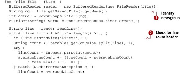
The filename can be used to tell which newsgroup each document belongs to . There is a header line that gives the number of lines, which can be encoded as a feature . Then, in parsing header lines and the body of the document , you need to count the words that you find. You can use a multi-set from the Google Guava library to do this counting. At least one of the documents has a bogus line count, and in that case it is reasonable to set the line count to the overall average to be defensive.

In each document, the headers come first and consist of lines containing a header name, a colon, content, and possible continuation lines that start with a space. The line number and the counts of the words on selected header lines are needed as features. After processing the headers, the body of the document is passed through the Lucene analyzer.

Vectorizing the Data

With the data from the document in hand, you’re ready to collect all of the features into a single feature vector that can be used by the classifier learning algorithm. Here’s how to do that:

Vector v = new RandomAccessSparseVector(FEATURES);
bias.addToVector(null, 1, v);
lines.addToVector(null, lineCount / 30, v);
logLines.addToVector(null, Math.log(lineCount + 1), v);
for (String word : words.elementSet()) {
  encoder.addToVector(word, Math.log(1 + words.count(word)), v);
}

First, encode the bias (constant) term, which always has a value of 1. This feature can be used by the learning algorithm as a threshold. Some problems can’t be solved using logistic regression without such a term.

The line count is encoded both in raw form and as a logarithm. The division by 30 is done to put the line length into roughly the same range as other inputs so that learning will progress more quickly.

The body of the document is encoded similarly except that the weight applied to each word in the document is based on the log of the frequency of the word in the document, rather than the straight frequency. This is done because words occur more than once in a single document much more frequently than would be expected by the overall frequency of the word. The log of the frequency takes this into account.

Measuring Progress So Far

At this point, you should have a vector and be ready to give it to the learning algorithm. Until then, the document can still be considered to be withheld data. And as such, you might as well use the data to get some feedback about the (hopefully improving) accuracy of the classifier. You can compute two measures of accuracy: the log likelihood and the average rate of correct classification.

Log likelihood has a maximum value of 0, and random guessing with 20 alternatives should give a result of close to –3. Log likelihood gives credit even when the classifier gets the wrong answer if the right answer is near the top, and it takes credit away if it gets the right answer but has a wrong answer with nearly as high a score. These close-but-not-quite properties of log likelihood make it a useful measure for performance testing. But it can be difficult to explain log likelihood to non-technical colleagues, so it’s good to have a simpler measure, the average rate of correct answers, as well.

You can compute the averages of the performance metrics using a trick known as Welford’s algorithm, which allows you to always have an estimate of the current average. A variant on Welford’s algorithm is used here, so that until you have processed 200 examples, a straight average is used. After that, exponential averaging is used so that you get a progressive measure of performance that eventually forgets about the early results from before the classifier had learned anything.

Here’s a snippet that calculates the log likelihood and average percent correct:

double mu = Math.min(k + 1, 200);
double ll = learningAlgorithm.logLikelihood(actual, v);
averageLL = averageLL + (ll - averageLL) / mu;

Vector p = new DenseVector(20);
learningAlgorithm.classifyFull(p, v);
int estimated = p.maxValueIndex();

int correct = (estimated == actual? 1 : 0);
averageCorrect = averageCorrect + (correct - averageCorrect) / mu;

In this snippet, the model is asked for some performance metrics. The model computes the average log likelihood in the variable averageLL. Then the most highly rated newsgroup is determined in the estimated variable, and it’s compared to the correct value. The result of the comparison is averaged to get the average percent correct as averageCorrect.

Training the SGD Model with the Encoded Data

After getting progress information from the current training example, you can pass it to the learning algorithm to update the model. If the algorithm is making multiple passes through the data, it’s probably a good idea to use testing examples for progress monitoring and training examples only for training, rather than using both types of examples for both training and progress monitoring, as we’ve done here.

In the example code, we used some fancy footwork to provide progress feedback at progressively longer intervals. This gives you fast feedback early in the run but doesn’t flood you with data if you let the program run a long time. Here is how these progressively longer steps are computed:

learningAlgorithm.train(actual, v);
k++;
int bump = bumps[(int) Math.floor(step) % bumps.length];
int scale = (int) Math.pow(10, Math.floor(step / bumps.length));
if (k % (bump * scale) == 0) {
  step += 0.25;
  System.out.printf("%10d %10.3f %10.3f %10.2f %s %s
",
       k, ll, averageLL, averageCorrect * 100, ng,
       newsGroups.values().get(estimated));
}
learningAlgorithm.close();

Each time the number of examples reaches bump * scale, another line of output is produced to show the current status of the learning algorithm. As the learning progresses, the frequency of status reports will decrease. This means that when accuracy is changing more quickly, there will be more frequent updates.

The last step is to tell the learning algorithm that it’s done. This causes any delayed learning to take effect and cleans up any temporary structures.

14.5. Choosing an algorithm to train the classifier

The main advantage of Mahout is its robust handling of extremely large and growing data sets. The algorithms in Mahout all share scalability, but they differ from each other in other characteristics, and these differences offer different advantages or drawbacks in different situations. Table 14.3 compares the algorithms used for classification within Mahout. This table, along with the rest of this section, will help you decide which Mahout algorithm bests suits a particular classification problem. Keep in mind that Mahout has additional algorithms not listed here—new ones continue to be developed.

No. 14

Table 14.3. Characteristics of the Mahout learning algorithms used for classification

Size of data set	Mahout algorithm	Execution model	Characteristics
Small to medium (less than tens of millions of training examples)	Stochastic gradient descent (SGD) family: OnlineLogisticRegression, CrossFoldLearner, AdaptiveLogisticRegression	Sequential, online, incremental	Uses all types of predictor variables; sleek and efficient over the appropriate data range (up to millions of training examples)
	Support vector machine (SVM)	Sequential	Experimental still; sleek and efficient over the appropriate data range
Medium to large (millions to hundreds of millions of training examples)	Naive Bayes	Parallel	Strongly prefers text-like data; medium to high overhead for training; effective and useful for data sets too large for SGD or SVM
	Complementary naive Bayes	Parallel	Somewhat more expensive to train than naive Bayes; effective and useful for data sets too large for SGD, but has similar limitations to naive Bayes
Small to medium (less than tens of millions of training examples)	Random forests	Parallel	Uses all types of predictor variables; high overhead for training; not widely used (yet); costly but offers complex and interesting classifications, handles nonlinear and conditional relationships in data better than other techniques

The algorithms differ somewhat in the overhead or cost of training, the size of the data set for which they’re most efficient, and the complexity of analyses they can deliver.

14.5.1. Nonparallel but powerful: using SGD and SVM

As you saw in figures 13.1 and 13.7 (in chapter 13), the behavior of an algorithm can be powerfully scalable even if the algorithm is nonparallel. This section provides an overview of two sequential Mahout learning algorithms, stochastic gradient descent (SGD) and support vector machine (SVM).

The SGD Algorithm

Stochastic gradient descent (SGD) is a widely used learning algorithm in which each training example is used to tweak the model slightly to give a more correct answer for that one example. This incremental approach is repeated over many training examples. With some special tricks to decide how much to nudge the model, the model accurately classifies new data after seeing only a modest number of examples. Although SGD algorithms are difficult to parallelize effectively, they’re often so fast that for a wide variety of applications, parallel execution isn’t necessary.

Importantly, because these algorithms do the same simple operation for each training example, they require a constant amount of memory. For this reason, each training example requires roughly the same amount of work. These properties make SGD-based algorithms scalable in the sense that twice as much data takes only twice as long to process.

The SVM Algorithm

An experimental sequential implementation of the support vector machine (SVM) algorithm has recently been added to Mahout. SVM implementations in Mahout include Java translations of the industrial-strength but nonscalable LIBLINEAR, which was previously only available in C++. The SVM implementation is still new and should be tested carefully before deploying.

The behavior of the SVM algorithm will likely be similar to SGD in that the implementation is sequential, and the training speed for large data sizes will probably be somewhat slower than SGD. The Mahout SVM implementation will likely share the input flexibility and linear scaling of SGD and thus will probably be a better choice than naive Bayes for moderate-scale projects.

14.5.2. The power of the naive classifier: using naive Bayes and compleme- entary naive Bayes

The naive Bayes and complementary naive Bayes algorithms in Mahout are parallelized algorithms that can be applied to larger data sets than are practical with SGD-based algorithms, as indicated in table 14.3. Because they can work effectively on multiple machines at once, these algorithms will scale to much larger training data sets than will the SGD-based algorithms.

The Mahout implementation of naive Bayes, however, is restricted to classification based on a single text-like variable. For many problems, including typical large data problems, this requirement isn’t a problem. But if continuous variables are needed and they can’t be quantized into word-like objects that could be lumped in with other text data, it may not be possible to use the naive Bayes family of algorithms.

In addition, if the data has more than one categorical word-like or text-like variable, it’s possible to concatenate your variables together, disambiguating them by prefixing them in an unambiguous way. This approach may lose important distinctions because the statistics of all the words and categories get lumped together. Most text classification problems, however, should work well with naive Bayes or complementary naive Bayes.

Tip

If you have more than ten million training examples and the predictor variable is a single, text-like value, naive Bayes or complementary naive Bayes may be your best choice of algorithm. For other types of variables, or if you have less training data, try SGD.

If the constraints of the Mahout naive Bayes algorithms fit your problem, they’re good first choices. They’re good candidates for data with more than 100,000 training examples, and they’re likely to outperform sequential algorithms at ten million training examples.

14.5.3. Strength in elaborate structure: using random forests

Mahout has sequential and parallel implementations of Leo Breiman’s random forests algorithm as well. This algorithm trains an enormous number of simple classifiers and uses a voting scheme to get a single result. The Mahout parallel implementation trains the many classifiers in the model in parallel.

This approach has somewhat unusual scaling properties. Because each small classifier is trained on some of the features of all of the training examples, the memory required on each node in the cluster will scale roughly in proportion to the square root of the number of training examples. This isn’t quite as good as naive Bayes, where memory requirements are proportional to the number of unique words seen and thus are approximately proportional to logarithm of the number of training examples.

In return for this less desirable scaling property, random forests models have more power when it comes to problems that are difficult for logistic regression, SVM, or naive Bayes. Typically these problems require a model to use variable interactions and discretization to handle threshold effects in continuous variables. Simpler models can handle these effects with enough time and effort by developing variable transformations, but random forests can often deal with these problems without that effort.

Now that you’re familiar with the learning algorithm options Mahout offers for training classifiers, it’s time to put that knowledge to work. You’ve already used the SGD algorithm to train a classifier for the 20 newsgroups data in section 14.4; in the next section we use a different algorithm for the same problem, and you’ll be able to compare the results of the two approaches.

14.6. Classifying the 20 newsgroups data with naive Bayes

The route to classification depends in part on the Mahout classification algorithm used. Whether the algorithm is parallel or sequential, as described in the preceding section, makes a big difference. The parallel SGD algorithm and the sequential naive Bayes algorithm have different input paths, and this difference requires different approaches to the handling of data, particularly with regard to vectorization.

This section will show you how to train a naive Bayes model on the same 20 newsgroups data set that you used in section 14.4. By using a different algorithm on the same data, you’ll see the differences between sequential and parallel approaches to building a classification model.

We’ll first go through the data extraction step needed to get the data ready for the training algorithm, and then you’ll learn how to train the model. Once that’s done, you’ll be ready to begin the process of evaluating your initial model to determine whether it’s performing well or changes need to be made.

14.6.1. Getting started: data extraction for naive Bayes

Let’s get the data into a classifiable form and convert it to a file format for use with the naive Bayes algorithm. You can use the same 20 newsgroups data set you downloaded for the SGD example in section 14.4.

The naive Bayes classifiers can be driven programmatically, as you did with the SGD classifier, but it also has a parser built in that can be invoked from the command line. This parser accepts a variant on the data file format used by the SVMLight program, in which each data record consists of a single line in the file. Each line contains the value of the target variable followed by space-delimited features, where the presence of the feature name indicates that the feature has a value of 1 and absence indicates that the feature has a value of 0. In order to use the command-line version of the naive Bayes classifier, you’ll have to reformat the data in the 20 newsgroups data set to be in this format.

The data in the 20 newsgroups data set has one directory per newsgroup, and inside each directory there’s one document per file. You need to scan each directory and transform each file into a single line of text that starts with the directory name and then contains all the words of the document. The Mahout program called prepare20newsgroups does just this. To convert the training and test data, use a command like this:

$ bin/mahout prepare20newsgroups -p 20news-bydate-train/ 
       -o 20news-train/ 
       -a org.apache.lucene.analysis.standard.StandardAnalyzer 
       -c UTF-8

no HADOOP_CONF_DIR or HADOOP_HOME set, running locally
INFO: Program took 3713 ms

$ bin/mahout prepare20newsgroups -p 20news-bydate-test 
       -o 20news-test 
       -a org.apache.lucene.analysis.standard.StandardAnalyzer 
       -c UTF-8
no HADOOP_CONF_DIR or HADOOP_HOME set, running locally
INFO: Program took 2436 ms

In this command, the –p option specifies the name of the directory holding the training or test data. The –o option specifies the output directory. The –a option specifies the text analyzer to use, and the –c option specifies the character encoding that should be used to convert the input from bytes to text.

The result should be a directory called 20news-train that contains one file per newsgroup. Inside a data file like 20news-train/misc.forsale.txt, you’ll see something like what is shown in figure 14.7.

Figure 14.7. Converted training data in the format preferred by the naive Bayes program. Note that the lines displayed here have been shortened considerably.

14.6.2. Training the naive Bayes classifier

Up to this point, you’ve been working with the 20 newsgroups data, extracting features to prepare the data appropriately for input to the naive Bayes algorithm. With the training and test data converted to the right format, you can now train a classification model.

Try this command to produce a trained model using the naive Bayes algorithm:

bin/mahout trainclassifier -i 20news-train 
            -o 20news-model 
            -type cbayes 
            -ng 1 
            -source hdfs
...
INFO: Program took 250104 ms

The result is a model stored in the 20news-model directory, as specified by the –o option. The –ng option indicates that individual words are to be considered instead of short sequences of words. The model consists of several files that contain the components of the model. These files are in a binary format and can’t be easily inspected directly, but you can use them to classify the test data with the help of the testclassifier program.

You have now built and initially trained a model using the 20 newsgroups data and the naive Bayes algorithm. How well is it working? You’re ready to address that question by beginning to evaluate the performance of your model.

14.6.3. Testing a naive Bayes model

It’s now time to evaluate the performance of your newly trained model. We just introduce the evaluation process here, and you’ll do some initial testing on your newly trained model. In chapter 15, we look at this topic in depth.

To run the naive Bayes model on the test data, you can use the following command:

bin/mahout testclassifier -d 20news-test 
            -m 20news-model 
            -type cbayes 
            -ng 1 
            -source hdfs 
            -method sequential

Here the –m option specifies the directory that contains the model built in the previous step. The –method option specifies that the program should be run in a sequential mode rather than using Hadoop. For small data sets like this one, sequential operation is preferred. For larger data sets, parallel operation becomes necessary to keep the runtime reasonably small.

When the test program finishes, it produces output like what follows. The summary has raw counts of how many documents were classified correctly or incorrectly.

...
Summary

-------------------------------------------------------
Correctly Classified Instances          :       6398    84.9442%
Incorrectly Classified Instances        :       1134    15.0558%
Total Classified Instances              :       7532
=======================================================

We’ve omitted some noisy output and just displayed the summary section from the output. Here, the naive Bayes model is performing well, with a score of nearly 85 percent correct. The summary doesn’t tell you anything about the errors that were made, other than the gross number. For more details about what errors were made, you can look at the confusion matrix in the next section of output, which appears something like this:

Confusion Matrix
-------------------------------------------------------
a b c d e f g h i j k l m n o p q r s t <--Classified as
388                                        | 397 a = rec.sport.baseball
  386                                      | 396 b = sci.crypt
    396                                    | 399 c = rec.sport.hockey
      347                                  | 364 d = talk.politics.guns
        377                                | 398 e = soc.religion.christian
  12      304           18                 | 393 f = sci.electronics
            281     14  43        21       | 394 g = comp.os.ms-windows.misc
              313       22 16              | 390 h = misc.forsale
     26 69      83 41                      | 251 i = talk.religion.misc
        45        225 13              11   | 319 j = alt.atheism
                    334           32       | 395 k = comp.windows.x
                      367                  | 376 l = talk.politics.mideast
          19 23 15      307 13             | 392 m =comp.sys.ibm.pc.hardware
                       16 335              | 385 n = comp.sys.mac.hardware
                            371            | 394 o = sci.space
                              393          | 398 p = rec.motorcycles
                             12 364        | 396 q = rec.autos
            11      22            305      | 389 r = comp.graphics
      102                           160    | 310 s = talk.politics.misc
                                      362  | 396 t = sci.med
Default Category: unknown: 20

Your output will look a little different because we squashed the actual output here to fit on shorter lines to fit on the page. The confusion matrix shows a complete breakout of all correct and incorrect classifications so that you can see what kinds of errors the model made on the test data. Along the diagonal, notice that most newsgroups are classified fairly well, although talk.religion.misc and talk.politics.misc both stand out somewhat because of the relatively smaller number of correct classifications. About a third of the documents from talk.politics.misc are incorrectly classified as belonging to talk.politics.guns, which is at least plausible if not correct. Likewise, 69 documents from talk.religion.misc are classified as soc.religion.christian, which is, again, plausible. It’s reassuring to see that the errors make a sort of sense, because that indicates that the model is picking up on the actual content of the documents in some meaningful way.

It’s also ironically reassuring to see that the performance of the model isn’t suspiciously good. For instance, if you run the same model on the same training data that it learned from, the summary looks like this:

bin/mahout testclassifier -d 20news-train -m 20news-model
   -type cbayes -ng 1 -source hdfs -method sequential
...
Correctly Classified Instances          :      11075    97.8876%
Incorrectly Classified Instances        :        239     2.1124%
Total Classified Instances              :      11314

When given this familiar data, the model is able to get nearly 98 percent correct, which is much too good to be true on this particular problem. The best machine learning researchers only claim accuracies for their systems around 84–86 percent. We talk more about how to evaluate models in later chapters and, in particular, how to develop an idea about how well the model really should be performing.

14.7. Summary

In working through this chapter, you’ve gained experience with building and training classifiers using real data from the 20 newsgroups data set. The chapter focused particularly on how to do feature extraction and how to choose the best algorithm for your particular project.

Feature extraction is a big part of building a classification system, both in time, effort, and the payoff of doing it well. Remember that not all features are equally useful for every classifier, and that you’ll need to try a variety of combinations to see what works. Raw data isn’t usable directly. You saw in detail how to process raw data into classifiable form and how to convert that into the vectors required by Mahout’s learning algorithms.

The types of values acceptable as input variables are different for the different learning algorithms, and section 14.5 provided an overview of those and other differences that distinguish one algorithm from another. You should now have a basic understanding of the benefits and costs of using the different algorithms to help guide you through making these choices in your own projects.

Finally, you saw the behavior of two different learning algorithms (SGD and naive Bayes) on the same data set, the 20 newsgroups.

Having learned a lot about the first stage of classification—training a model—you’re now ready to move on to the second stage—evaluating and tuning the performance of a trained model. Those are the topics of the next chapter.