Chapter 16. Deploying a classifier

This chapter covers

• Specifying the speed and size requirements of a classifier
• Building a large-scale classifier
• Delivering a high-speed classifier
• Building and deploying a working classification server

This chapter examines the issues you face in putting a classification system into real-world production. In previous chapters, we talked about the advantages of using Mahout classifiers when working with large data sets, how the classifiers are trained, how they work internally, and how you can evaluate them, but those discussions purposely omitted many of the ways that the real world intrudes when you need to put a classifier into production. In this chapter, we examine these real-world aspects as we explain how to deploy a high-speed classifier. We include tips on how to optimize feature extraction and vector encoding, describe how to balance load and speed requirements, and explain how to build a training pipeline for very large systems, such as those appropriate for Mahout classification. Finally, we provide an example of the deployment of a Thrift-based server that allows fully functional load-balanced classification.

If you’re planning to use Mahout in production, there’s a good chance that some or all of the following are true: you have a huge amount of training data, you have high throughput rates, you have fast response time requirements, or you need to integrate with a large pre-existing system. Each of these characteristics implies specific architectural and design considerations that you need to take into account as you build your system. Large data sets require efficient ingestion and organization; high throughput requires scalable and optimized code. Integration into large systems requires a simple and clean API that plays well as a networked service. Mahout offers a powerful way to deal with big data systems, but there are also ways to simplify or restate problems to make tools like Mahout even more powerful.

In the next section, we present an overview of how to design, build, and deploy a real-world large-scale classifier.

16.1. Process for deployment in huge systems

There are a few standard steps that will help ensure success when you deploy a Mahout-based classifier system. The key is to anticipate problems that may arise and then choose which ones you’ll put your primary efforts toward preventing. The detailed strategies for coping with each of these issues are explained in sections 16.2 through 16.4; in this section we introduce the process of deploying a huge system.

Note

To understand the potential value of Mahout for your classification project, look for aspects of your system that are especially large, or where you need it to be especially fast. Finding these pain points will tell you whether or not Mahout is the right solution.

The deployment process can be broken down into these steps:

• Scope out the problem
• Optimize feature extraction as needed
• Optimize vector extraction as needed
• Deploy the scalable classifier service

Each of these steps is described in this section and then put into practice in the examples that follow.

16.1.1. Scope out the problem

The first step is to determine how large a problem you actually have and how fast your system has to run in both training and production classification. The size of your training data dictates whether feature extraction will allow use of conventional tools, like a relational database, or whether you’ll need to put some effort into building a highly scalable feature extraction system using tools like Apache Hadoop. The specifics of size and speed requirements will be explored in section 16.2.

The allowable time for training will determine whether you can use a sequentially trained classifier such as SGD at all. Here’s why. With a parallel algorithm and limited time for training, you can add more machines if your system isn’t fast enough to process larger amounts of data. But if you use a sequential training algorithm, you’ve got a budget of one computer for a fixed time. To make this work with large amounts of data, you may have to put extra effort into making the parsing and encoding of data particularly efficient.

The throughput and latency requirements for the production classifier will determine whether you need a distributed classifier and whether you need to do extensive precomputation and currying to maximize classification speed. For utmost throughput at some cost in latency, you may also decide to do batch classification.

16.1.2. Optimize feature extraction as needed

As data sizes get to be more than tens of millions of examples, it becomes more and more important to use scalable techniques such as MapReduce for feature extraction.

At small to medium scale—up to a few million examples—any technique will work, and proven data management and extraction technologies like relational databases will serve well.

As scale increases, you’re likely to have to commit to a parallel extraction architecture, such as Hadoop, or a commercially supported system like Aster Data, Vertica, or Greenplum. If you choose to use Hadoop, you’ll also have to decide what general approach you’ll use to implement your feature extraction code. Good options include Apache Hive (http://hive.apache.org/), Apache Pig (http://pig.apache.org), Cascading (http://www.cascading.org/), or even raw MapReduce programs written in Java.

A key point here is that any downsampling should be done as part of feature extraction rather than vector encoding so that it can be done in parallel. Issues in real-world feature extraction for big data systems are examined in detail in section 16.3.

16.1.3. Optimize vector encoding as needed

If you have less than about 100 million training examples per classifier after feature extraction and downsampling, consider a sequential model builder such as SGD. If you have more than about five million training examples, you’ll also need to optimize your data parsing and feature vector encoding code fairly carefully. This requirement may involve parsing without string conversions, multithreaded input conversion, and caching strategies to maximize the speed with which data can be fed to the learning algorithm.

For more than about 10 million training examples, you may want to consider using a CrossFoldLearner directly with predefined learning-rate parameters. If the problem is relatively stable, you may be able to use an adaptive technique to learn good learning-rate schedules and then just stick with what works well. The advantage of doing this over using an AdaptiveLogisticRegression is that 20 times fewer numerical operations are required in learning. The disadvantages are that the speedup isn’t nearly as large as it sounds, and your learning chain will require more maintenance.

16.1.4. Deploy a scalable classifier service

In most applications, it’s convenient to separate classifiers into a distinct service that handles requests to classify data. These services are typically conventional services based on a networked RPC protocol such as Apache Thrift or REST-based HTTP. An example of how to build a Thrift-based classification server is shown in section 16.4. This is particularly appropriate where many classification operations are done on each input example, such as where many items are tested for expected value.

In a few cases, the network round trip is an unacceptable overhead and the classifier needs to be integrated as a directly called library. This happens when very small-grained requests must be done at extreme rates. Because it’s possible to achieve throughputs of over 50,000 requests per second with modern network service architectures, such cases are relatively rare.

16.2. Determining scale and speed requirements

The first step in building a classifier is to characterize the scale factors, including the amount of training data and the throughput rates that your system is required to meet. Knowing the size of the problem in various dimensions will in turn lead to several design decisions that will characterize how your system will need to be built.

16.2.1. How big is big?

If you’re considering using Mahout to build a classification system, ask yourself these questions about your system and use the answers to determine which parts of your system will require big-data techniques and which can be handled conventionally:

• How many training examples are there?
• What is the batch size for classification?
• What is the required response time for classification batches?
• How many classifications per second, in total, need to be done?
• What is the expected peak load for the system?

These values need not be estimated exactly. Typically, numbers that are within an order of magnitude are good enough for initial system scaling and architecture. As you move into production, you’ll be able to refine the estimates for final tuning.

Once you have an idea of the number of training examples you expect to use, you can consider whether or not Mahout is appropriate for your project, and if so, which algorithms are likely to be a good choice.

Implications of the Number of Training Examples

Typically, Mahout becomes interesting once you exceed 100,000 training examples. There is, however, no lower bound on how much data can be used. When you have 10 million or more training examples, most other data-mining solutions are unable to complete training, whereas above 100 million or a billion training examples there are very few systems available that can build usable models. The number of training examples, along with model types, are the primary determinants of the training time.

With a scalable system such as Mahout, you can extrapolate fairly reliably from smaller tests to determine expected training time. With sequential learning algorithms such as SGD, learning time should scale linearly with input size. In fact, many models converge to acceptable error levels long before all available input has been processed, so training time grows sublinearly with input size.

With parallel learning algorithms such as naive Bayes, learning time scales roughly linearly with input size divided by the number of MapReduce nodes available for learning. Because naive Bayes learning is coded as a batch system where all input is processed through multiple phases, it can’t be stopped early. This means that even though a partial data set might be sufficient to produce a useful model, all training examples must be processed before a usable model is available.

Classification Batch Size

It’s common for a number of classifications to be done to satisfy a single request. This requirement often occurs because multiple alternatives need to be evaluated. For instance, in an ad placement system, there are typically thousands of advertisements that each have models to be evaluated to determine which advertisement to show on a web page. The batch size in this case would be the number of advertisements that need to be evaluated. A few applications have very large batches of more than 100,000 models.

At the other extreme, a fraud-detection server might only have a single model whose value needs to be computed, because the question of whether a single transaction is fraudulent involves only one decision: fraud or not fraud. This situation is very different from an advertisement-selection server, where a click-prediction model must be computed for each of many possible advertisements.

Maximum Response Time and Required Throughput

The maximum response time determines how quickly a single batch of classifications must be evaluated. This, in turn, defines a lower bound on the required classification rate. This rate is only a lower bound because if there are enough transactions per second, it may be necessary to support an even higher rate.

Typically, it’s pretty easy to build a system that supports 1,000 classifications per second with small classification batch sizes because such a rate is small relative to what current computers can do. In fact, the Thrift-based server described later in this chapter can easily meet this requirement. Until batch sizes exceed 100 to 1,000 classifications per batch, you should be able to support roughly that transaction rate, because costs will be dominated by network time. At batch sizes of 10,000 or more, response times will start to climb substantially. At larger batch sizes and with subsecond response times required, you’ll probably need to start scaling horizontally or restructuring how the classifications are done.

16.2.2. Balancing big versus fast

One of the advantages of using Mahout is that the trade-offs between large data and fast operation are much looser than in nonscalable systems. That said, there is almost always a trade-off to some extent between these characteristics of a system, so you’ll need to consider how to balance these needs. To do this, keep in mind that one aspect of your system may have different requirements than another. It’s common to use different classifiers for different purposes in the same system.

Once you have the overall characteristics of your system in mind, you can begin to outline those aspects of your deployment that will require special attention and which can be implemented more quickly. The following sections outline the most important considerations in each phase of the deployment. These considerations generally apply either during training or after deployment, during classification.

At Training Time

Running the large-scale joins necessary to create classifiable data often dominates all other aspects of training. You can use standard Hadoop tools for that, but care needs to be taken to make the joins run efficiently.

Downsampling negative cases can help enormously by making your training data much, much smaller. In fraud or click-through optimization, the number of uninteresting training examples typically vastly outnumbers the number of interesting ones (the frauds or clicks). It’s critical to accurate learning that you keep all of the interesting records, but many of the uninteresting records can often be randomly discarded as long as you keep enough to still dominate the interesting records. This discarding is called downsampling and is usually done as part of the joining process.

Feature encoding often dominates training time after you have your training examples. Downsampling the training data helps reduce the encoding time, but there are still a number of things you can do to make the encoding process itself more efficient.

Through it all, it’s important to remember that building good classification models requires many cycles of iterative refinement. You need to make sure your training pipeline makes these iterations efficient. Section 16.3 covers the architectural and tactical issues involved in building a training pipeline.

At Classification Time

When you come to integrating your classifier into your system, your overall classification throughput needs will drive your selection of what you need to optimize in the classifier. Most Mahout classifiers are fast enough that this will only matter in extreme systems, but you need to check whether you’re in the extreme category. If not, you’re ready to roll with the standard methods, but if you’re extreme, you’ll need to budget time to stretch the normal performance limits.

If you need to do small numbers of classifications per transaction and have only modest latency and throughput requirements, it should suffice to use a conventional service design with a single thread per transaction. REST-based services may be acceptable, or you may need to use a somewhat higher-performance network service mechanism like Thrift, Avro, or Protocol Buffers. Section 16.5 has an example of how to build such a service.

If you require a moderate number (10s to 1000s) of classifications per evaluation and have more stringent latency and throughput requirements, you’ll need to augment the basic classification service with a multithreaded evaluation of multiple models or inputs, but otherwise the basic design should still suffice.

For extreme batch sizes with very large numbers of model computations per service transaction, you’ll need to dive into the heart of the model evaluation code in order to divide the model evaluation into portions that can be evaluated ahead of time and portions that must be evaluated at classification time. Details of such optimizations are highly specific to your particular application and are largely beyond the scope of this book. An example of such an implementation using Mahout is given in chapter 17.

16.3. Building a training pipeline for large systems

Classifications systems need training data, and scalable classification systems can eat truly enormous amounts of data. In order to feed these systems, you have to be able to process even larger volumes of data in order to pick out the bits that you can use to train your classifier.

In order to handle these huge volumes of data, there are a few things to keep in mind. The first and most important is to match your techniques to your task. If you have less than about a million training examples, for instance, almost any reasonable technique will work, including conventional relational databases or even scripts that process flat-file representations of your data. At 100 million training examples, relational databases can still do the necessary data preparation, but getting the data out becomes progressively more and more painful. At a billion examples and beyond, relational databases become impractical, and you’ll probably have to resort to MapReduce-based systems like Apache Hadoop.

A billion training examples sounds extreme, but it’s surprisingly common to reach that level. Shop It To Me, the company we profile in chapter 17, for example, sends several million emails each day, each containing hundreds of items. As a result, they generate several hundred million training examples per day, a number that rapidly turns into billions of training examples. The larger ad networks all have well above a billion ad impressions per day, each of which is a potential training example. A music streaming service with a million unique visitors per month can produce nearly a billion training examples each month.

No matter what your volume, your model-training data pipeline will need to support the following capabilities:

• Data records will have to be acquired and stored coherently, typically in time-based partitions.
• Data records will have to be augmented by joining against reference data of some kind.
• Data records will need to be joined to target variable values.
• Downsampling of training data may be useful and should be supported.
• Other kinds of filtering and projection beyond simple downsampling will be required.
• Training records will need to be encoded as training features.
• Trained models will have to be retained and associated with metadata describing how to encode input records.

The various parts of the training data pipeline can usually scale horizontally, but when it comes to training a model, some of the most easily deployed kinds of Mahout models aren’t suitable for horizontal scaling for the training process. This means that at very high data volumes, early cleaning and processing of data can be done in a highly scalable fashion, but significant efforts may be necessary to make data encoding very efficient for when the model is actually trained.

This section will cover the most important aspects of how to build these capabilities into your data pipeline using Mahout and related technologies. We focus next on techniques that you can use at large scales on the assumption that you’ll already be familiar with the techniques that you can use at smaller data scales.

16.3.1. Acquiring and retaining large-scale data

Training a large-scale model means that you’re going to have to deal with really big sets of training data. As always, issues that are trivial with small-scale data often balloon to magnificent and dire proportions when working with large-scale data. Most of these problems arise from the fact that large-scale data has a significant amount of what is metaphorically called inertia. This inertia makes it hard to move or transform large-scale data and requires that you plan out what you intend to do. In the absence of direct experience with a new class of data, this planning is impossible to do effectively. Instead, you have to fall back to following standard best practices until you have enough experience with your data.

Acquiring Data

The first problem with large data sets is acquiring them. This sounds easy, but as with all things to do with large-scale data resources, it’s harder than it looks. The primary issue at this level is to keep the data relatively compact and to maintain natural parallelism inherent in the production of the data.

For instance, if you have a farm of servers each handling thousands of transactions per second, it’s probably a bad idea to use a single centralized log server. Excessive concentration is bad because it leaves you liable to single-point failures, and because it’s very easy for backpressure from the data acquisition system to adversely affect the operation of the system being observed. To avoid this problem, it’s crucial to build load shedding into the data acquisition phase; it’s preferable to lose data than for your production system to crash.

The second trick to acquiring large data sets is to make sure that you keep data intended for machines to read in machine-readable form. It’s nice to have human-readable logs, but extracting data from such logs is a common source of errors because of the fairly loose format. It’s better to keep some data in human-readable form for humans to read and to keep the data you want to process in machine-readable formats.

For large-scale data ingestion, there are a number of different data formats that can be used, but only a few that provide the necessary combination of compactness, fast parsing libraries, and, most important, schema flexibility. Schema flexibility allows you to evolve the data that you store without losing the ability to read old data.

The two most prominent encoding formats that combine these features are Avro from Apache and Protocol Buffers from Google. Both are well supported and both provide comparable features and flexibility. Storing data in comma- or tab-separated fields is common, but this approach quickly leads to problems as schemas evolve, due to confusion about which column of data contains which field. The confusion becomes especially severe when files with differing schemas must be handled concurrently.

Partitioning and Storing Data

As you acquire and store data, there are several organizing principles that need to be maintained to ensure that you wind up with a scalable system:

• Directories should generally contain no more than a few thousand files. Larger directories can cause scaling problems because opening and creating files will begin to take longer with very large directories.
• Programs should process as few files as possible, which can be achieved by not processing irrelevant data and by keeping files as large as practical. Avoiding irrelevant data limits the amount of data to be transferred, and using large files minimizes the time lost due to disk seeks, thus maximizing I/O speed.
• The directory structure used to organize files should support your most common scheme for selecting relevant training data. Organizing directories well allows you to find relevant files without sifting through all of your files.
• Files should not generally be more than about 1 GB in size to facilitate handling them. Files should be small enough that you can transfer them between systems in a reasonably short period of time. This limits the impact of network disruption by allowing you to repeat transfers quickly. About 1 GB is a happy middle ground.

Following these principles generally leads to storing data with top-level directories that define the general category of data and with subdirectories that contain data from progressively finer time divisions.

Tip

It’s generally good practice to concatenate small older files into larger files that represent large enough time periods to avoid excessively many input files for subsequent processing. If fine-grained time resolution is required for recent time periods, then files might be kept for very short periods, such as five minute intervals, but beyond a few days, these should be accumulated into hourly and then into daily files. If the data for a single day totals more than 1–2 GB, keeping several files for each day is probably a good idea.

Working Incrementally

For the most part, feature extraction isn’t something that requires aggregation over long periods of time. That means that once you have done the necessary joins and data reduction to generate the corresponding training data for an hour’s worth of data, that training data will probably not change when the next hour of data comes in. This characteristic makes it eminently feasible to collect training data incrementally rather than doing all feature extraction for the entire period of interest each time training is done.

Likewise, this incremental processing makes it possible to accumulate extracted features for short periods of time and then concatenate them for longer-term storage. It’s common, for instance, to accumulate hourly training data and concatenate these hourly training files into dailies that are then kept pretty much forever. This corresponds nicely to the way that the raw data is usually kept.

When your classification system is relatively new, the addition of new features and changes in downsampling will likely mean that you’ll need to rebuild your training data files fairly often. Over time, the frequency of change typically decreases. Once this happens, creating training data incrementally is a big win because the lag between the arrival of data and the beginning of model training can be decreased.

16.3.2. Denormalizing and downsampling

It’s common for the data that you acquire directly to require denormalization before it can be used to train a model, because the original data may be scattered across many different storage formats including log files, database tables, and other sources. In denormalization, data that could be less redundantly stored in separate tables connected by keys is joined together so that each record is self-contained without any references to external data, such as user profile tables or product description tables.

Because model training algorithms have no provision for resolving external references, their inputs have to be fully denormalized to be useful.

Denormalization is almost always done using some kind of join. With small to medium data sets, almost any method will suffice to do these joins, and tools such as relational databases are very useful. With large datasets, however, these joins become much more difficult to do efficiently. Moreover, the characteristics of your data must be taken into consideration to do these joins.

Join Target First

Joins are also almost universally required to attach target variable values to predictor variables. The target values should be attached, if possible, before denormalization, because it’s common to downsample training records depending on the value of the target variable. By downsampling before any subsequent joins, it’s often possible to achieve substantial savings during training, because less data is processed with almost identical results.

In-Memory Joins

In some cases, training data needs to be joined to a secondary table with a limited number of rows. When this is the case, the secondary table can sometimes be loaded into memory, and the join can be done by consulting an in-memory representation of the second table.

The in-memory table is loaded in the configure method of the mapper or reducer. In-memory joins can be done inside a MapReduce program as part of either the mapper or the reducer, although when you’re generating classification training data, map-side joins are more common.

In-memory joins are called memory-backed joins in some references, such as Jimmy Lin and Chris Dyer’s book, Data-Intensive Text Processing with MapReduce.

Merge Joins

Where both data sets to be joined are large, a merge join may be possible. In a merge-join in a sequential, non-parallel program, two data sets ordered on the same key can be joined in a single pass over both data sets.

In a MapReduce program, the situation is a bit more complex because the two data sets are very unlikely to be split in such a way that each map can merge data correctly. It’s possible, however, to build an index on one file while sorting it. The path of the indexed data is provided as side data so that as each map starts reading a split of the unindexed data, it can seek to near the right place in the indexed data and start merging from that point.

Merge joins are advantageous when data is naturally sorted, but it’s often overlooked that if only one of the inputs is sorted and indexed, then a merge join can be done in the reducer instead of in the mapper. This choice allows you to use the MapReduce framework to sort the unindexed input. Whether this approach saves time relative to a full reduce join is something that can only be determined by experimentation.

Full Reduce Joins

In terms of programming effort, the simplest way to join data is to do a full reduce join. This means that you simply read both inputs in the mapper and reduce on the key of interest. Such joins can be more expensive than merge joins because more data needs to be sorted in the Hadoop shuffle step.

When you do a full reduce join, it helps to have Hadoop sort the results so that the training records come after the data being added to the training records to denormalize them. Having Hadoop do the sort allows the reducer to be written in a fully streaming fashion. Because the shuffle and sort in Hadoop are highly optimized, a brute-force full reduce join may be as efficient as a merge join, if not more so, especially if you’re doing a reduce side merge join.

If your training data is larger than the data it’s being joined to, a full reduce join and any kind of merge join are likely to be comparable in speed.

16.3.3. Training pitfalls

Even assuming that your data is what you think it is, your joins are working correctly, and you’re parsing your data correctly, there are a few pitfalls that are very easy to run into. The most subtle and difficult to diagnose is a target leak. Also common is the use of an inappropriate encoding, which leads to a semantic mismatch between what you intended and how the model sees the data. Let’s look at these issues in more detail.

Target Leaks

Keeping daily training files substantially facilitates time-shifted training, which is often necessary to avoid target leaks.

For instance, suppose one feature that you want to use in a targeting system is a clustering of users based on click history. If you use that clustering to train a model on the same time periods that you used to derive the clustering, you’ll probably find that the resulting model will do exceedingly well at predicting clicks. What’s happening, however, is that your click-history clustering is probably putting everybody with no clicks into different clusters than everybody with clicks. This division means that the user cluster is a target leak in the time period when the clustering was created.

A picture of how such a target leak can creep into your design is in figure 16.1. To fix this leak, you can’t just delete the problematic variable. The user-history clustering could still be a valuable predictive variable. The problem here is simply that the model isn’t being trained on new data.

Figure 16.1. Don’t do this: click-history clustering can introduce a target leak in the training data because the target variable (Clicks > 0) is based on the same data as the cluster ID.

Figure 16.2 shows how this can be improved by clustering data from early time periods and then training on more recent data unknown to the clustering algorithm. Moreover, the withheld test data can be from even more recent time periods.

Figure 16.2. A good way to avoid a target leak: compute click history clusters based on days 1, 2, and 3, and derive the target variable (Clicks > 0) from day 4.

Keeping data segregated by time makes holding back test data very easy. In this scenario, you would use data from day 5 as withheld data to evaluate model performance.

Semantic Mismatch During Encoding

A rose by any other name would still smell as sweet, but with training data, an integer isn’t always what it seems. In some cases, an integer represents a quantity such as the number of hours or days between two events. In other cases, integers are used as identifiers for categories. The distinction between these cases has been covered in previous chapters, but in spite of the best intentions, it’s still common for integer data to be treated incorrectly when training models. This mistake can be hard to debug, because a model built with incorrectly encoded data may actually be able to perform correctly a surprising amount of the time.

The key to diagnosing such problems is to review the internal structure of the resulting model to look for a few weights applied to each field. If you see lots of weights for particular values of a field, the field is being treated as an identifier for a categorical or word-like value. If you see a single weight for the field, it’s being treated as a continuous variable. Whichever way the model is thinking of the field should match the way you think of the field.

The one exception to this sort of rule is when you have integer values that really are integers, but which only have a few distinct values. Treating such variables as having a categorical value may be useful even if they’re more correctly treated as having a continuous value. Only experimentation can really determine if this will work for you, but whenever you have integers with a small number of values, this trick may be worth trying.

16.3.4. Reading and encoding data at speed

For many applications, the methods for reading, parsing, and encoding data as feature vectors that were discussed in previous chapters are good enough. It’s important to note, however, that the SGD classifiers in Mahout only support training on a single machine rather than in parallel. This limitation can lead to slow training times if you have vats of training data. Look at a profiler and you’ll see that most of the time used in the Mahout SGD model training API is spent in preparing the data for the training algorithm, not in doing the actual learning itself.

To speed this up, you have to go to a lower level than is typical in Java programs. The String data type, for instance, is handy in that it comes with good innate support for Unicode and lots of libraries for parsing, regex matching, and so on. Unfortunately, this happy generality also has costs in terms of complexity. It’s common for training data to be subject to much more stringent assumptions about character set and content than is typical for general text.

Another major speed bump that training programs encounter is a copying style of processing. In this style, data is often processed by creating immutable strings that represent lines of input. These lines are segmented into lists of new immutable strings representing input fields. Then, if these fields represent text, they’re further segmented into new immutable strings during tokenization. The tokens in the text may be stemmed, which involves creating yet another generation of immutable strings.

Doing all of the allocations involved in such a copy-heavy programming style costs quite a bit, and lots of people focus on reducing allocation costs by reusing data structures extensively. The real cost, however, isn’t so much the cost of allocation, but the cost of copying the data over and over. An additional cost is due to the fact that constructing a new String object in Java involves creating the hash code for each new string. Computing the hash code costs almost as much as copying the data.

All of this copying provides an opportunity to increase speed enormously by working at a lower level of abstraction and avoiding all of these copies. In this lower-level style, if you do allocate new structures, you should try to make sure that they reference the original data rather than a copy. These small structures are also highly ephemeral, so the cost of allocating and collecting them is nearly zero.

As an example of a string copying style, here’s a simple class that uses strings to parse tab- or comma-separated data. This class illustrates a simple, clear, and somewhat slow approach to parsing this kind of data:

class Line {
  private static final Splitter onTabs = Splitter.on(SEPARATOR);
  private List<String> data;
  private Line(String line) {
    data = Lists.newArrayList(onTabs.split(line));
  }
  public double getDouble(int field) {
    return Double.parseDouble(data.get(field));
  }

}

Obviously, important details are left out here, but the key idea is clear. The class splits a string representation of a line into a list of strings. This splitting and allocating of new strings requires that you copy the data around repeatedly. Moreover, by copying strings, you’re copying two bytes per character.

The following listing shows how this code could be used to parse and encode data from a file containing CSV data.

Listing 16.1. Code to parse and encode CSV data

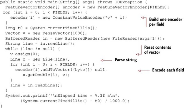
This code reads each line, one at a time, and parses each line using the Line class shown earlier. For each field that’s found, a feature encoder is used to add the field to the feature vector. Separate encoders are used for each field. When used to parse a million lines, each with 100 data elements, the string style of parsing and encoding shown in listing 16.1 takes 75 to 80 seconds running on a 2.8 GHz Core Duo processor. If you make a few changes, you can speed this up by a factor of at least 5. With the improvements we’re about to describe, a program that does the same work takes well under 15 seconds.

Segment Bytes, Not Characters

The first step to speed things up is to use large-scale byte I/O, and not to convert bytes to Strings, and definitely to avoid copying pieces of the input over and over. In the Line class, each line is copied from the input, then copied again when it’s converted to a string, and then copied again as the pieces are parsed out. All of this copying makes the program easier to understand and to debug, but it definitely slows things down quite a bit.

For many data files, avoiding the conversion to Java strings is a fine thing to do because the files generally have a limited data format that can be expressed in an ASCII character set, where each character is encoded by a single byte code. Java characters are twice as large as bytes, and moving them around requires twice as much memory bandwidth. Even better, with byte arrays, you have the option to avoid copies almost entirely. If the fields in question contain numbers, using the normal Java primitives means that the fields will be parsed by routines that are capable of converting general Unicode strings into numbers. This conversion is harder than it sounds because basic digits appear many times in Unicode. If your data is all ASCII, the conversion can be done a lot more simply than by converting your data to Unicode and then converting such a general representation to a number.

Listing 16.2 shows an adaptation of the Line class called FastLine that uses a ByteBuffer to avoid copies. This code can also be found as an inner class in the SimpleCsvExamples program in the Mahout examples module. FastLine also parses numbers in a way that’s highly specialized for parsing one- and two-digit integers encoded in an ISO-Latin character set.

Listing 16.2. Code for byte-level CSV parsing

The FastLine class in listing 16.2 uses IntArrayLists from the Mahout collections package to store offsets and lengths. This has two effects. One is to avoid the boxing and unboxing of integers. A second effect is that fields are kept as references into the original byte array to avoid a copy.

The parsing of the file data is based on several strong assumptions that depend on the input data being somewhat constrained. First, there’s an assumption that the ByteBuffer always has enough data in it to complete the current line. Second, the data is assumed to use Unix-style line separators consisting of a newline character with no carriage return character. Thirdly, it’s assumed that only the ASCII subset of characters is used.

These assumptions allow considerable liberties to be taken, with the result that the time required for reading and parsing the data is less than one-third the time required for the same operations in the String-based code. FastLine is good, but it isn’t the whole story.

Direct Value Interface to Value Encoders

Values can be encoded as vectors in a number of ways. For continuous variables, you can use the ContinuousValueEncoder and pass in the value as a string, as you saw in previous chapters. On the other hand, if you already have the desired value in the form of a floating-point number, you can pass in a null as the string and pass in the value in the form of the weight.

In the case of a direct byte parser, you can have access to the value of the field very quickly without converting to a string and then to a floating-point representation. This makes the shortcut use of the weight field on the ConstantValueEncoder attractive. The following code shows how this can be done.

Listing 16.3. Direct value encoding

This code is similar to the string-oriented encoding code, except for the use of FastLine instead of Line. The same encoders are constructed and lines are still read, but from a FastLine instead of from a string level input. The encoding of each field is a bit different because the FastLine class converts the byte representation to a number, to avoid letting the encoder do the job.

The final version of the code using FastLine is about five times faster, as was mentioned earlier, but the effect of this direct value-encoding trick in isolation is even more impressive. For the million lines, ignoring the time required for data parsing, it takes about 4–5 seconds to encode all of the values when they’re extracted from the byte representation, but it takes over 40 seconds to encode the values from string form.

The overall effect of these speedups is that raw data to be classified can be read, parsed, and encoded at a rate of about 15 MB/s without much effort. By using several threads for reading, the aggregate conversion rate can easily match disk transfer speeds for several spindles. With more elaborate encodings including lots of interaction variables, the cost of encoding will be higher, but these improvements will still have large impacts.

Such optimizations are worthwhile if you’re running large modeling runs, especially if you’re using a lower level CrossFoldLearner or OnlineLogisticRegression object directly, without the mediation of an AdaptiveLogisticRegression, because these lower-level learners are so fast that reading the training data can be the limiting factor on performance. On the other hand, using the more abstracted string-based methods allows you to write code that’s much easier to write and debug and much less prone to surprises if your data files have oddities in them.

Once you have your data read (quickly) and converted (quickly), the next performance bottleneck is likely to be integrating your classifier into a server.

16.4. Integrating a Mahout classifier

Integrating a Mahout classifier is usually just a matter of creating a simple networked service. As such, the general issues of throughput, latency, and service updates that apply to all networked services apply to a Mahout classifier service. These issues can take on a slightly different hue with Mahout classifiers than is customary because Mahout classifiers are often integrated into applications that require extreme speed. But to some extent, services based on Mahout classifiers are simpler than most services because they’re stateless. This statelessness allows trivial horizontal scaling.

This section will cover how to plan and execute the job of integrating a Mahout classifier into a service-based architecture. Then in section 16.5 these ideas are pulled together into a complete working example classification server.

16.4.1. Plan ahead: key issues for integration

Although Mahout-based services have the advantage of being simple, you should still consider some key things when creating such a service in order to use Mahout to its full potential. These key issues include best practices about the division of responsibility for the client and server, checking production data for differences from training data, designing for speed, and handling model updates.

Dividing Responsibilities

One of the critical architectural choices you’ll face as you integrate classification models into a classification service is the division of responsibilities between the client and server sides of your system. A well-considered division can greatly enhance performance and will help future-proof your design.

In general, it’s important to ensure that the server handles the encoding of features and evaluation of the model. There’s a gray area, however, in how much feature extraction should be done on the client or server sides. For instance, if the client has a user ID and a page URL, but the server needs information from the user’s profile and some content features based on the content of the page, then either the client or the server can do the necessary join against the user profile database and a page content or feature cache. Doing these join and feature-extraction operations on the client side will leave the model server with a much more circumscribed task and will likely result in a more reliable server. Doing these join and extraction operations on the server side will make certain kinds of caching easier and will hide the details of the model from the client a bit more.

Figure 16.3 illustrates how the responsibilities can be divided.

Figure 16.3. Joins with profile data, such as user profiles, are preferably done on the server, but these joins may be done by the client. Feature encoding should definitely be done on the classification server.

It’s a good design principle for the model server to accept whatever form of data the client programs already have. If possible, the model server shouldn’t require extensive data preparations to be done by the client unless they were already being done before the model service existed. A major exception to this principle is when providing the model server access to join resources would create a need for access to secured resources that are already available to the client. In such a case, joins that are necessary in preparation for feature encoding may have to be done by the client.

Real-Time Features are Different

One major issue with deploying a model into production is that the data that’s given to a classifier in production is often quite different from the data that’s reconstructed for training a classifier. These differences are generally not intentional, and they can lead to subtle bugs and apparent poor performance of the classifier system if not handled properly.

What sort of differences are you likely to encounter? Some of these differences are due to time-shifting processes, similar to target leaks. For instance, suppose you’re trying to predict whether a user will purchase a particular product, and the predictor variables for the problem are based on the contents of the user’s profile. In creating the training data for this model, it would be easy to collect user profiles as they are at the time the training data is collected rather than as they were at the time the purchase decision was made. If the completion of the purchase process results in additional information being stored in the user profile, any model built using the time-shifted profiles is likely to behave very poorly when given non-shifted profiles.

Logging Requests

One of the best ways to detect when production data differs from training data is to log all classification requests even before the classification system is ready for deployment. After a short period of logging, you can use any technique you prefer to extract training data for the period of time in question, and compare the logged data with the extracted data. If they differ, the training data extraction process must somehow be changed to avoid extracting time-shifted training examples. Ultimately, it may be that only directly logged data can be used for training.

Designing for Speed

Speed considerations when building a classification system often go to paradoxical extremes. When a Mahout classifier is properly integrated, extreme speeds are definitely achievable. If your service is evaluating a single model against a single input record, and the classification server doesn’t have to do any expensive joins, the model evaluation is likely to be so fast that network overheads will dominate. The speed problem will reduce to simply finding an access method that can drive high volumes of requests through the server.

For instance, a Thrift server running locally takes a bit less than 50–100 μs to do a server request, no matter how little the request actually does. Because a typical model evaluation requires no more than a thousand or so floating-point operations, it will finish in a few tens of microseconds at most, resulting in 90 percent of the time being spent in overhead. The throughput will be a bit higher than this due to threading and network transit time, but it’s clear that most of the time isn’t spent on model evaluation. In such a system, the key place to put your effort is in optimizing network latency. To achieve the highest speed, you may need to integrate the model directly into your client code, avoiding server round trips entirely. This direct integration minimizes latency for each model evaluation, but it may substantially complicate model updates.

Tip

If you need to evaluate one example at a time, focus on decreasing network round trip times to minimize evaluation latency, and consider client-side model evaluation. For model updates, you may need some kind of server to simplify the distribution of model updates rather than depending on the file being accessible as a local file.

In the middle of the speed spectrum, some uses of classifier models require many models to be evaluated at a time, or allow many feature vectors to be sent together in a single server request. This batched evaluation approach can allow substantial increases in efficiency by virtue of the fact that network latency is amortized over more model computations. Latency isn’t decreased relative to the case with a single evaluation per server request, but the amount of computation that can be done per request is increased dramatically.

Note

Doing lots of model evaluations per server request is a good thing, especially in terms of throughput. Many targeting systems require model evaluations for lots of items and thus allow this optimization.

At the extreme end of the speed spectrum, systems typically have enormous numbers of inputs to be evaluated. The computational marketing system described in the next chapter, for instance, requires that tens to hundreds of thousands of products be evaluated for each user, resulting in as many model evaluations as there are items. One request is made per user, and a feature vector is constructed using user parameters, item parameters, and user-item interactions. The models in that system are also fairly elaborate, involving hundreds or thousands of nonzero features for each item. In such cases, the evaluation time can be several hundred milliseconds, and computation time totally dominates all architectural decisions.

Coordinating Model Updates

In a production system that’s handling a stream of classification requests, it’s fairly common for there to be an expectation of nearly 100 percent uptime. Because a classifier is normally stateless, this uptime requirement can be satisfied by placing a pool of classification servers behind a load balancer. Whenever the classification model is updated and released to production, it’s necessary for the servers to load the new model and start using the new model for classification. In some cases, there is an additional requirement that model updates be made visible at essentially the same time across the entire pool of servers to maintain consistency among all servers.

Regardless of your exact requirements, we highly recommend using a coordination service to manage model updates and to provide a reliable list of live servers.

Among such services, Apache ZooKeeper is far and away the most popular, and we highly recommend it. ZooKeeper allows you to connect to a small cluster of servers that provide an API to access what looks a lot like an ordinary filesystem. In addition to very simple create, replace, and delete functions, however, ZooKeeper provides change notifications and a variety of consistency guarantees that simplify building reliable distributed systems even in the presence of server failures, maintenance periods, and network partitions.

A ZooKeeper-coordinated architecture for model updates can be quite simple, especially if exactly synchronized updates aren’t necessary. In this architecture, ZooKeeper holds a model configuration. Classification servers request notifications about changes to this configuration, and while they have a live model, they maintain indicator files that tell classification clients which servers are handling requests. Classification clients interrogate ZooKeeper to determine which classification servers are available.

This data in ZooKeeper can be arranged in the following directory structure:

/model-farm/
   model-to-serve
   current-servers/
     10.1.5.30
     10.1.5.31
     10.1.5.32

In this directory structure, the /model-farm/model-to-serve file contains the URL of the serialized version of the model that all servers should be using. Each live server reads this file on startup and tells ZooKeeper to provide notifications of any changes. In addition, each server should poll this file every 30–60 seconds in case notifications couldn’t be set, possibly because the file didn’t exist when the server was started.

When ZooKeeper notifies the server that a change to model-to-serve has been made, the server should download the serialized form of the model and instantiate a new model. This new model should then be used to serve all subsequent requests. Once the new model is properly installed, the server should create a file in the /model-farm/current-servers directory with a name unique to the server, and it should contain, either in the name or file contents, information necessary for a client to send requests to the server. Such information might include a host name and port number. Some care is warranted here to deal correctly with the case of machines with multiple network interfaces.

Figure 16.4 contains a ladder diagram showing a typical time sequence for the deployment of a new model.

Figure 16.4. How model deployments are coordinated with ZooKeeper. The control process, server1, and server2 all communicate via ZooKeeper, which also notifies server1 and server2 when changes happen.

In the sequence depicted in figure 16.4, we assume that ZooKeeper starts with a model specification. When server1 starts, it loads the specification from ZooKeeper and then loads the model. When the model is fully loaded and ready to serve, server1 creates a file in ZooKeeper to indicate that it’s ready. When server2 starts up a short time later, the same sequence ensues. When the control process updates ZooKeeper with a new model, notifications are passed to server1 and server2, and the model download and announcement process repeats.

This process is simple to understand and easy to implement. It has significant limitations, however, in that all servers run the same model, and all servers update their models essentially simultaneously. This simultaneous access could conceivably result in degraded service across the entire cluster because servers will switch to using the new model whenever they have completed the load process, which in turn could cause a short time when different servers will give different answers. Similarly, a server may have somewhat slower response time immediately after a new model is loaded, so having all servers in such a degraded state simultaneously may not be desirable. Also, if the model file is large, having all servers read it simultaneously could cause problems due to network overload.

Here is a directory structure that shows how updates can be coordinated so that a more cautious model update can be done:

/model-farm/
   should-load/
      node-10.1.5.30
      node-10.1.5.31
      node-10.1.5.32
      node-10.1.5.33
   currently-loaded/
      node-10.1.5.30
      node-10.1.5.31
      node-10.1.5.32
      node-10.1.5.33
   model-to-serve/
      node-10.1.5.30
      node-10.1.5.31
      node-10.1.5.32
      node-10.1.5.33

In this directory structure, the top-level model-farm directory is the name of the overall model cluster. Below this, the should-load directory contains a single file for each server named with the address of the server. The content of each of these files is a list of URLs and MD5 hashes that can be used to retrieve and verify the content of the model. Parallel to the should-load directory is the currently-loaded directory; it contains a single ephemeral file created by each active model server that contains a list of the MD5 hashes for all models that are currently loaded on that server. Finally, another sibling directory called model-to-serve contains one file per server node that contains the hash of the single model that should be used for all incoming requests.

In operation, each model server maintains a watch on the should-load directory and the model-to-serve file. Changes in the should-load directory signal that a model should be loaded or dropped, whereas changes to the model-to-serve file signal that all subsequent requests be routed to the indicated model. Whenever a model is loaded or unloaded, the corresponding ephemeral file in currently-loaded is updated.

This directory structure allows considerably more flexibility than the previous model at the cost of implementation complexity. This flexibility allows new models to be loaded and staged on multiple machines before making them available essentially simultaneously. It also allows you to load and run a new model on only one server in order to test the stability of the new model before rolling it out to all of the servers. The use of MD5 hashes allows the reuse of URLs with new content and allows servers to verify that they have loaded the intended model.

In practice, you may need to extend this model to control multiple model server farms or you may want to automate how models are rolled out to progressively more machines. It’s also common to have servers update their status files with indicators about how much traffic they can handle. Clients sending requests can use these indicators when picking a server to send a request to.

Also, keep in mind that even if you train your model using an AdaptiveLogisticRegression, which contains many models inside, you only need to save a single model from one of the underlying CrossFoldLearners. This is important because the AdaptiveLogisticRegression contains a large number of classifiers, each of which has a potentially very large coefficient matrix inside. With a large feature vector size, the size of a serialized AdaptiveLogisticRegression can actually be hundreds of megabytes.

16.4.2. Model serialization

As of version 0.4 of Mahout, the SGD and naive Bayes models are serialized in different ways. The SGD models share a helper class called ModelSerializer that handles the serialization and deserialization of all SGD models. In contrast, the naive Bayes models are only ever serialized as a side effect of the multiple files created during training. Deserialization of naive Bayes models isn’t done using a single method, but rather by reading these multiple files back into memory explicitly.

In future versions of Mahout, it’s likely that the ModelSerializer or a similar class will likely be extended to handle naive Bayes models as well as SGD-based models. Until then, the serialization and deserialization of naive Bayes models will remain a tricky and highly variable process. Until a more usable serialization interface is completed, this means that any deployment of a naive Bayes model should be done using the command-line interface we described in previous chapters rather than programmatically.

Using the Modelserializer for SGD Models

The ModelSerializer class provides static methods that serialize models to files and strings. The use of the class is quite simple, as shown in the following snippet, where both a single model from an AdaptiveLogisticRegression as well as the complete ensemble model are saved to different files:

if (learningAlgorithm.getBest() != null) {
   ModelSerializer.writeBinary("best.model",
      learningAlgorithm.getBest().getPayload().getLearner());
 }
 ModelSerializer.writeBinary("complete.model", learningAlgorithm);

All of the different kinds of SGD models can be serialized using the same approach.

Reading a model from a file is just as easy, as shown here:

learningAlgorithm = ModelSerializer.readBinary(
              new FileInputStream("complete.model"),
              AdaptiveLogisticRegression.class);

OnlineLogisticRegression bestSubModel = ModelSerializer.readBinary(
        new FileInputStream("best.model"), OnlineLogisticRegression.class);

In this snippet, two uses of a ModelSerializer are shown. The first might be used to reload an entire AdaptiveLogisticRegression, complete with submodels, whereas the second can be used to load a single OnlineLogisticRegression, which might be one of the component models in an AdaptiveLogisticRegression. Note how you have to supply the class to the readBinary method so that it can know what kind of object to construct and return.

When serializing SGD models for deployment as classifiers, it’s usually best to only serialize the best-performing submodel from an AdaptiveLogisticRegression. The resulting serialized file will be 100 times smaller than would result from serializing the entire ensemble of models contained in the AdaptiveLogisticRegression object. In addition, when data is to be classified, the individual model is more suited to deployment because only the best submodel from the AdaptiveLogisticRegression object would be used, and all of the other models would be ignored.

On the other hand, if you’re serializing a model so that you can continue training at a later time, serializing the entire AdaptiveLogisticRegression is probably a better idea.

16.5. Example: a Thrift-based classification server

Putting all the bits of a working classification server together can be a bit daunting. To help with that, this section contains a full working example that illustrates all that we’ve talked about. We’ve written a simplified, but complete, classification server that implements the simpler model deployment scheme described in section 16.4. This server provides all of the basic capabilities needed for a fully functional load-balanced classification service, including some administrative capabilities.

Communication between the classification client and server will be handled in this example using Apache Thrift (http://thrift.apache.org/). Thrift is an Apache project that allows client-server applications to be built very simply.

The coordination of multiple servers and between server and client will be handled in this example using Apache ZooKeeper (http://zookeeper.apache.org/). In this example, ZooKeeper holds instructions for all of the classification servers about which model to load, as well as status information from all of the servers so that the client can tell which servers are up and which model they’re serving. This server coordination structure is shown in figure 16.5.

Figure 16.5. ZooKeeper serves as a coordination and notification server between the classification client and server.

This arrangement allows the classification server to know where to find the model definition and allows the client to find all active servers.

When a server comes up, it queries ZooKeeper to find out what model to load. After loading that model, it announces to the world that it’s ready for traffic by writing a file into ZooKeeper. Whenever the file indicating which file to load is changed, ZooKeeper notifies all servers of the change.

When a client wishes to send a query to a server, it can look into ZooKeeper to find out which servers are currently providing service and pick one server at random.

The structure of the ZooKeeper files that coorTdinate everything is as follows:

/model-service/
   model-to-serve
   current-servers/
     hostname-1
     hostname-2

The file called model-to-serve contains the URL of the model that should be loaded and used for classification by all servers. These servers will maintain a watch on this file so that they’re notified as soon as it changes. When they see a change, they’ll load the file to get the model URL, and then they’ll reload the model. As soon as any model is loaded by a server, it will create an ephemeral file in the current-servers directory with the name of the server. Because this file is ephemeral, it will vanish within a few seconds if the corresponding server ever crashes or exits.

The code for the main class of this model server is shown in listing 16.4. It mostly contains the setup code for the Thrift server layer, but note how a timer is used to schedule periodic checks in ZooKeeper. This should be completely redundant, but it’s a good example of belt-and-suspenders coding style. ZooKeeper should notify you of any changes, but checking in now and again makes sure you’ll catch up if something gets lost due to a programming error.

Listing 16.4. Main program for the classification server

Most of the action is in the modelWatcher object . This object is an implementation of a ZooKeeper Watcher, and it’s invoked whenever a watch is triggered by the modification of the model-to-serve file. Here’s the source code for the modelWatcher.

Listing 16.5. The watcher object loads the model and sets model status

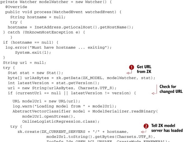
A lot of this code exists to handle exceptional conditions, but the basic outline is quite simple. The backbone of the code is in the calls to zk.getData , zk.create , and zk.setData .

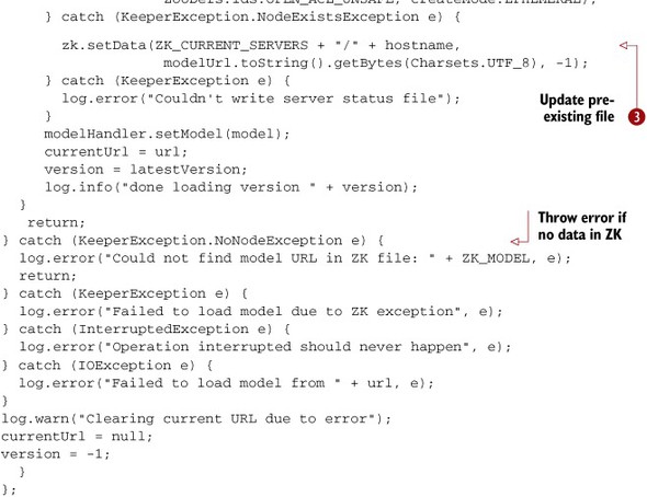
The way the code works is that it attempts to read the URL of the model from ZooKeeper. If a URL is read but there is no current model, or if the version of the ZooKeeper file containing the URL is different from the one for the current model, the model is reloaded and the status file for this server is updated with the model URL. The update is done by first trying to create the status file, and if that fails to update the status file.

If the original read of the URL failed due to the model file being missing, a message is logged and a relatively normal return ensues. Other errors cause the server to null out the URL of the current model to make sure that it reloads the model at the next opportunity.

The actual handling of classification requests is done by a Thrift server. The interface is defined in Thrift IDL as shown here:

namespace java com.tdunning.ch16.generated
service Classifier {
  list<double> classify(1: string text)
}

This interface definition declares that the server will accept classification requests. Each request will return a list of scores, one for each possible value of the target variable.

The interface defined by the preceding IDL is implemented in the Ops class, which is shown next.

Listing 16.6. Implementation of classification service

The classify method classifies a feature vector using the currently loaded model. This method is called by the Thrift server when a client request is received and encodes the text passed to it in the style of the TrainNewsGroups program in chapter 15. The model is then used to compute a vector of scores, and these scores are returned.

The Ops class also defines a setModel method that the ZooKeeper watcher class can use to load a new model when a model change is observed.

16.5.1. Running the classification server

To see this server in action, you can use the command-line interface to ZooKeeper to instigate behaviors. Before you start, though, you need a model to work with. TrainNewsGroups, from listing 15.3 in chapter 15, is a handy program to get such a model from because it writes a copy of a model to /tmp every few hundred training examples.

The process of setting up and running the TrainNewsGroups components is described in the README file with the source code.

When you run the TrainNewsGroups program, the result is a mass of output. The critical bits of the output are shown here:

[INFO] [exec:java {execution: default-cli}]
11314 training files
0.62 189992.00 ... 7000  -1.017 81.02 none
0.64 189992.00 ... 8000  -0.898 84.77 none
0.75 189997.00 ... 10000 -0.948 84.71 none
...

As a side effect, you get model files stored in /tmp:

$ ls -l /tmp/
-rw-r--r--  1 ...  1680247 Nov 21 01:16 news-group-1000.model
-rw-r--r--  1 ...  1680247 Nov 21 01:16 news-group-1200.model
-rw-r--r--  1 ...  1680247 Nov 21 01:16 news-group-1400.model
-rw-r--r--  1 ...  1680247 Nov 21 01:16 news-group-1500.model
...
-rw-r--r--  1 ...  1680247 Nov 21 01:19 news-group.model
$

The files with names like news-group-*.model contain the best model at each stage of learning.

Once you have some model files, you can start a local copy of ZooKeeper as described in the instructions in the README file from the Chapter 16 source code.

With ZooKeeper running, you can start the classification server:

...
10/11/21 01:36:06 INFO zookeeper.ClientCnxn: Socket connection established to
     localhost/fe80:0:0:0:0:0:0:1%1:2181, initiating session

10/11/21 01:36:06 WARN ch16.Server: Starting server on port 7908
...
10/11/21 01:36:07 ERROR ch16.Server: Could not find model URL in ZK file: /
     model-service/model-to-serve
10/11/21 01:36:08 WARN ch16.Server: Starting server on port 7908
...

This is best done in a separate window from the one used to start ZooKeeper so that you can separate the different log lines as they come out.

At this point, the classification server is running, but there is nothing in ZooKeeper to tell it what model to load and use to classify requests. To put the right things into ZooKeeper, you can use the ZooKeeper command-line interface, as shown next. Again, a new window is helpful to keep things separated.

$ ~/Apache/zookeeper/bin/zkCli.sh  <<EOF
create /model-service ""
create /model-service/model-to-serve 
           file://localhost/tmp/news-group-1500.model
quit
EOF

These commands should produce lots of output, most importantly including lines like this:

[zk: 1] Created /model-service
[zk: 3] Created /model-service/model-to-serve

As you were talking to ZooKeeper, the classification server you started earlier was checking every 30 seconds to see if ZooKeeper was correctly set up. Each time it did so, it would emit the same error message about not being able to find the model URL. On the cycle after you finally create the /model-service/model-to-serve file, however, it will produce a different message:

10/11/21 01:45:04 INFO ch16.Server: Loading model from file://localhost/tmp/
     news-group-1500.model
10/11/21 01:45:04 INFO ch16.Server: model loaded

At this point, the classification server is up and running. You can watch it respond to configuration commands in ZooKeeper by changing the content of the model-to-serve file:

~/Apache/zookeeper/bin/zkCli.sh  <<EOF
set /model-service/model-to-serve file://localhost/tmp/xxx.model 
quit
EOF

Almost instantly after doing this, you’ll see the server output a warning that it can’t find this bogus model. You can put things right again with this command:

~/Apache/zookeeper/bin/zkCli.sh  <<EOF
set /model-service/model-to-serve 
      file://localhost/tmp/news-group-1500.model
quit
EOF

Almost instantly, the classification server will respond with a confirmation that it has loaded the model. If you had 10 model servers running on different machines, they would all respond just as quickly.

16.5.2. Accessing the classifier service

On the client side, matters are even simpler. The following listing shows how the client can get information from ZooKeeper to find out what servers are live and then request one of them to do the desired classification.

Listing 16.7. Accessing the sample classification server

The first thing that the client does is contact ZooKeeper to get a list of the live servers and picks one at random . After that, it connects to the randomly selected server and requests the server to classify two bits of text .

The output of the client program should look like this when you run it, with some bits omitted here for clarity:

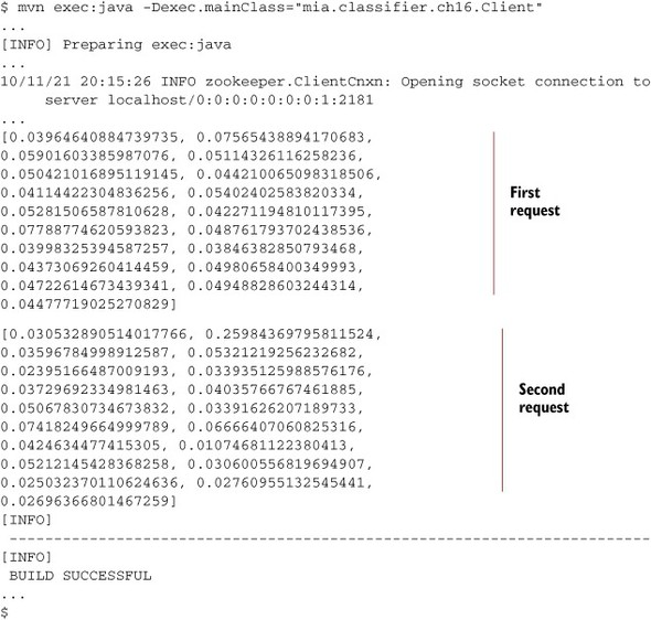
The output from the two requests appears as a list of numbers, each of which is the score of a different newsgroup. The second request is the more interesting one because it has text that was extracted from an actual newsgroup posting. That request also shows a significantly higher score for the second newsgroup, as you would expect when giving a classifier some data it can make a decision about.

Clients written like this example inherently balance the load across multiple servers. Moreover, a slightly more advanced client that’s written to perform multiple queries in sequence can maintain a watch on the current servers directory on ZooKeeper. Whenever the watch is triggered, the client can pick an alternative server. This will cause immediate load rebalancing as soon as any new server comes online or shortly after a live server exits or crashes.

This Apache Thrift-based server example isn’t quite ready for prime time, but you should be able to take it as a skeleton for many kinds of real-world production deployments. A key aspect of the design of this system is the use of ZooKeeper for coordination and notification between the classification client and server in a system with multiple servers. This approach allows the classification server to scale quickly and transparently and to change which models are live at any time.

16.6. Summary

Congratulations! You’ve successfully navigated the third and final stage in Mahout classification, deploying a large-scale classifier. Now you know how to build and train models for a classification system, how to evaluate and fine-tune your models to improve performance, and how to deploy the trained classifier in huge systems. Some key lessons learned from this chapter regarding deployment include the importance of fully scoping out the project, paying particular attention to any parts of your system that, as designed, could exceed what Mahout can easily do. Discovering these potential difficulties ahead of time gives you the chance to modify your design to avoid the problems or to budget time to stretch those boundaries.

Often the most intense aspect of deploying a large-scale system is building the training pipeline. In systems of the size you’ll tackle with Mahout, the pipeline may offer some substantial engineering challenges. One key to doing this successfully is what you have learned about doing extremely large-scale joins to implement the pipeline in parallel.

The chapter also showed you some of the pitfalls to avoid: namely, how not to produce target leaks or create a semantic mismatch. We showed several subtle ways that these leaks can occur and how you can avoid them.

The final lessons you have learned involve the service design. In this chapter you have seen the core design of a robust classification service based on standard technologies like ZooKeeper and Thrift. If you keep the spirit of this service design, you should be able to deploy high-performance classification services reliably and repeatably. But don’t be fooled by the simplicity of the design presented in this chapter. Much of the simplicity, robustness, and reliability of this system are provided by building on the firm foundation of ZooKeeper. Reflect carefully before you diverge too far from this basic design idea.

As you saw, deploying even a well-designed classifier is a complicated task when it’s integrated into a larger system. We’ll conclude our exploration of classification in the next chapter, which puts all of this together in presenting a real-world case study of a large-scale classification system used by an online marketing company, ShopItToMe.