
Chapter 12. Real-world applications of clustering
- Clustering like-minded people on Twitter
- Suggesting tags for an artist on Last.fm using clustering
- Creating a related-posts feature for a website
You probably picked up this book to learn and understand how clustering can be applied to real-world problems. So far we’ve mostly focused on clustering the Reuter’s news data set, which had around 20,000 documents, each having about 1,000 to 2,000 words. The size of that data set isn’t challenging enough for Mahout to show its ability to scale. In this chapter, we use clustering to solve three interesting problems on much larger data sets.
First, we attempt to use the public tweets from Twitter (http://twitter.com) to find people who tweet alike using clustering. Second, we examine a data set from Last.fm (http://last.fm), a popular Internet radio website, and try to generate related tags from the data. Finally, we take the full data dump of a popular technology discussion website, Stack Overflow (http://stackoverflow.com), which has around 500,000 questions and 200,000 users. We use this data set to implement related-features functionality for the website.
Our first problem is finding similar users by clustering tweets from Twitter.
12.1. Finding similar users on Twitter
Twitter is a social networking and micro-blogging service where people broadcast short, public messages known as tweets. These tweets are at most 140 characters long. Once posted, a tweet is instantly published on the feed of all of the user’s followers and it’s visible publicly on Twitter’s site. These tweets are sometimes annotated with keywords in a style like #Obama or marked as directed at another user with syntax like @SeanOwen.
Because Twitter’s new terms of service don’t allow us to publish data sets, you’ll need to prepare it yourself. In the book’s source code, there’s a class called TwitterDownloader that grabs 100,000 tweets from Twitter (though you can change this number in the source code) and writes them to a file that later will be used for analysis. Fetching 100,000 tweets will take about 2 hours.
Note
To run this program, you’ll need to obtain an authentication key from Twitter by registering your application at https://dev.twitter.com/apps, and putting the authentication values into the program, as described in the source code. And don’t forget to add the -Dfile.encoding=UTF-8 option when you run this program—otherwise you’ll lose all non-ASCII characters.
12.1.1. Data preprocessing and feature weighting
This data must be preprocessed to put it into a format usable by Mahout. First it must be converted to the SequenceFile format that can be read by the dictionary vectorizer. Then this must be converted into vectors using TF-IDF as the feature-weighting method.
The dictionary vectorizer expects its input to have a Text key and value. Here, the key will be the Twitter username, and the value will be the concatenation of all tweets from that user.
Preparing this input is a job well suited to MapReduce. A Mapper reads each line of the input: username, timestamp, and the tweet text separated by tabs. It outputs the username as the key and the tweet text as the value. A Reducer receives all tweets from a particular user, joins them into one string, and outputs this as the value, with the username again as the key. This data is written into a SequenceFile.
The Mapper, the Reducer, and the Configuration classes, along with a Job that invokes them on a Hadoop cluster, are shown in listings 12.1 and 12.2. The Map-Reduce classes are implemented as a generic group-by-field Mapper.
Listing 12.1. Group-by-field mapper

Listing 12.2. Group-by-field reducer

Once the job executes, the user’s tweets are concatenated into a document-sized string and written out to the SequenceFile. Next, this output must be converted to TF-IDF vectors. Before running the dictionary-based vectorizer, it’s worth understanding the Twitter data set better and identifying some simple and helpful tweaks that will aid the feature-selection and weighting process.
12.1.2. Avoiding common pitfalls in feature selection
TF-IDF is an effective feature-weighting technique that we’ve used several times already. If it’s applied to individual tweets, most term frequencies would be 1 because the text is 140 characters in length, or perhaps 25 total words. We’re interested in clustering users that tweet alike, so we’ve instead created a data set where a document consists of all the tweets for a user, instead of individual tweets. Applying TF-IDF to this will make more sense, and the clustering will happen more meaningfully.
Directly applying TF-IDF weighting may not produce great results. It would be better to remove features that commonly occur in all tweets: stop-words. We use the dictionary vectorizer and set the maximum document frequency percentage parameter to a low value of perhaps 50 percent. This removes words that occur in more than 50 percent of all documents. We also use the collocations feature of the vectorizer to generate bigrams from the Twitter data and use them as features for clustering.
But there is a problem. Tweets are casually written messages, not carefully edited text like that in the Reuters news collection. Tweets contain misspellings, abbreviations, slang, and other variations. Three people tweeting the sentences below will never get clustered together because their tweets have no words in common:
HappyDad7: "Just had a refreshing bottle of Loke"
BabyBoy2010: "I love Loca Kola"
Cool_Dude9: "Dude me misssing LLokkkeee!!!!"
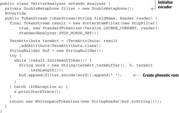
To solve this problem, we can discover the relationship between these alternate spellings using phonetic filters. These are algorithms that reduce a word to a base form that approximates the way the word is pronounced. For example, Loke and Loca might both be reduced to something like LK. The word refreshing could be reduced to something like RFRX. There are at least three notable implementations of a procedure like this: Soundex, Metaphone, and Double Metaphone. All are implemented in the Apache Commons Codec library.[1] We use its DoubleMetaphone implementation to convert each word into a base phonetic form. The following listing shows a sample Lucene Analyzer implementation using DoubleMetaphone in this way.
1 You can find the hierarchy for the Apache Commons Codec package at http://commons.apache.org/codec/apidocs/org/apache/commons/codec/language/package-tree.html
Listing 12.3. Lucence Analyzer class optimized for Tweets
Note
The DoubleMetaphone filter will only work for English text. You might need to find a filter if you deal with other languages. When you’ll grab tweets from Twitter, the collection will also contain tweets in other languages. We ignore the quality loss due to other languages for this example.
Copy the SequenceFile generated in section 12.1.1 to the cluster using the Hadoop HDFS copy command. Once the data is copied to the cluster, you can run the DictionaryVectorizer on the Twitter SequenceFiles as follows:
bin/mahout seq2sparse -ng 2 -ml 20 -s 3 -x 50 -ow
-i mia/twitter_seqfiles/ -o mia/twitter-vectors -n 2
-a mia.clustering.ch12.TwitterAnalyzer -seq
It’s important to make sure the TwitterAnalyzer class is in the Java CLASSPATH when you try to run this command. Vectorization may take some time to tokenize the tweets and generate the complete set of bigrams from them. The vectorized representation will be smaller than the original input.
We don’t know the number of clusters we need to generate. Because fewer than 100,000 unique users generated those tweets, we can decide to create clusters of 100 users each, and generate around 1,000 clusters. Run the k-means algorithm using the vectors you just generated. An example of a cluster from the output we got when we ran this is listed below:
Top Terms:
        KMK                     =>    7.609467840194702
        APKM                    =>   7.5810538053512575
        TP                      =>    6.775630271434784
        KMPN                    =>    5.795418488979339
        MRFL                    =>   4.9811420202255245
        KSTS                    =>    4.082704496383667
        NFLX                    =>    4.005469512939453
        PTL                     =>   3.9200561702251435
        N                       =>   3.7717770755290987
        A                       =>   3.4771755397319795
Here the feature KMK is the output of the DoubleMetaphone filter for words like comic, comics, komic, and so on. To see the original words, run the clustering with vectors without using any of the filters, or simply using the StandardAnalyzer.
You can rerun clustering twice more with the maximum document frequency set at 50 percent and at 20 percent. When we did so, the following top-terms lists were selected from the cluster containing tweets about the topic comics:
Top Terms with -maxDFPercent=50
        comic                   =>    9.793121272867376
        comics                  =>    6.115341078151356
        con                     =>    5.015090566692931
        http                    =>    4.613376768249454
        i                       =>    4.255820257194115
        sdcc                    =>    3.927590843402978
        you                     =>    3.635386448917967
        rt                      =>   3.0831371437419546
        my                      =>   2.9564724853544524
        webcomics               =>    2.916910980686997

Top Terms with -maxDFPercent=20
        webcomics               =>   11.411304909842356
        comic                   =>   10.651778670719692
        comics                  =>   10.252182320186071
        webcomic                =>    7.813077817644392
        con                     =>    5.867863954816546
        http                    =>    4.937416185651506
        companymancomic         =>    4.899269049508231
        spudcomics              =>    4.543261228288923
        rt                      =>    4.149479137148176
        addanaccity             =>    4.056342724391392
These two sets of output illustrate the importance of feature selection in a noisy data set like tweets. With the maximum document frequency set at 50 percent of the document count, there are features like i, you, my, http, rt. These features dominate the distance-measure calculations, so they appear with higher weights in the cluster centroid. Decreasing the document-frequency threshold removed many of these words. Still, there are words like http and rt that appear in the second cluster, which should ideally be removed. But setting a much lower threshold runs the risk of removing important features. The best option is usually to manually create a list of words and prune them away using the Lucene StopFilter: words like bit.ly, http, tinyurl.com, rt, and so on.
This is clustering using only words to calculate user similarity. But similarity can also be inferred from user interaction. For example, if user A retweeted (forwarded, or repeated) user B’s tweet, you might count B as a feature in A’s user vector, with a weight equal to the number of times A retweeted B’s tweets. This may be a good feature for clustering users who think alike.
Alternatively, if the feature weight were the number of times the users mentioned each other in a tweet, adding this as a feature might negatively affect the clustering result. Such a feature is best for clustering people into closed communities that tweet with each other, and not for clustering users who think alike. The best feature for one problem may not be good for others.
The clustering result will show how various tech bloggers are clustered together and how various friend groups are clustered together. We leave it to you to inspect the results and experiment with the clustering. Next, we take a look at another interesting problem: a tag-suggestion engine for a web 2.0 radio station.
12.2. Suggesting tags for artists on Last.fm
Last.fm is a popular Internet radio site for music. Last.fm has many features; of interest here is a user’s ability to tag a song or an artist with a word. For example, the band Green Day could be tagged with punk, rock, or greenday. The band The Corrs might be tagged with words like violin and Celtic.
We now try to implement a related-tags function using clustering. This could assist users in tagging items; after entering one tag, the system could suggest other tags that seem to go together with that tag in some sense. For example, after tagging a song with punk, it might suggest the tag rock. We explore how to do this in two ways: first, with a simple co-occurrence–based approach, and then with a form of clustering.
We use as input a data set that records the number of times each artist was tagged with a certain word. The data set is available for download from the web at http://musicmachinery.com/2010/11/10/lastfm-artisttags2007/. It contains raw tag counts for the 100 most frequently occurring tags that Last.fm listeners have applied to over 20,000 artists during that period. The data set has this format:
artist-id<sep>artist-name<sep>tag-name<sep>count
Each line in the data set contains an artist ID and name, a tag name, and the count of times that tag was applied to the artist.
12.2.1. Tag suggestion using co-occurrence
We can use co-occurrence, or the number of times two tags appear together for some artist, as the basis of a similarity metric between tags. We saw co-occurrence first in chapter 6, where we counted item co-occurrence. With a similarity metric, we can then cluster.
For each tag, we could count co-occurrence with all other tags and present the most co-occurring tags as suggestions. There is only one problem. A frequently occurring tag like awesome will co-occur with many other tags, so it would become a suggestion for many tags, even though it isn’t a particularly helpful suggestion. From that perspective, we might have to cut out high-frequency tags.
This technique, however, will never suggest tags that are two or more hops away. That is, if tag A co-occurs with B and B co-occurs with C, this method won’t suggest tag C to the person adding tag A. A workaround is to add all the tags that are two hops away from tag A to the suggestion list, and rerank the tags.
But clustering takes care of this out of the box. If the tags are within a certain distance threshold, regardless of whether they co-occur together, they’re clustered.
We can model this problem as artist-based clustering where the artist is the document and the feature is the tag the artist receives. Alternatively, you can think of tags as documents, the artists as words in the document, and the number of times they co-occur as the word frequency. These are alternative views of the same problem and can be modeled like a bipartite graph as shown in figure 12.1.
Figure 12.1. A typical bipartite graph (a graph where nodes can be put in one of two partitions). Here, one type of node is for artists and the other is for tags. The edges carry a weight equal to the number of times a tag was applied to the artist. In the world of recommenders, the nodes were users and items, and the edge weights denoted the star ratings. Recommenders and clustering algorithms are more closely related than many people realize.

The Last.fm data set already looks like it can be directly converted to vectors. We create a simple vectorizer that first generates a dictionary of artists, and, using the dictionary, convert the artists into integer dimensions in a MapReduce fashion. We could have used the strings as IDs, but Mahout Vector format only takes integer dimensions. The reason for converting artists into integer dimensions will be clear once we arrive at the code that vectorizes Last.fm artists into vectors of their tags.
12.2.2. Creating a dictionary of Last.fm artists
To generate these feature vectors for the Last.fm data set, we employ two MapReduce jobs. The first generates the unique artists in the form of a dictionary, and the second generates vectors from the data using the generated dictionary. The Mapper and Reducer classes of the dictionary generation code are shown in listings 12.4, 12.5 and 12.6.
Listing 12.4. Output artists from the data set

The Mapper takes a line of text and outputs the artist as the key with an empty value. This is passed into the reducer.
Listing 12.5. Grouping by artist and outputting a unique key-value pair for an artist

The Mapper emits the artist, and the Reducer emits only a unique artist and discards the list of empty strings. Once the dictionary is generated, it can be read into a HashMap, which maps the words to a unique index as the value, as shown in the following listing. This is done sequentially.
Listing 12.6. Using the unique artist names to create a unique integer ID for each artist

This HashMap is serialized and stored in the Hadoop configuration. It then goes into the next Mapper, which uses this as a dictionary to convert string tags to integer dimension IDs, as you’ll see next.
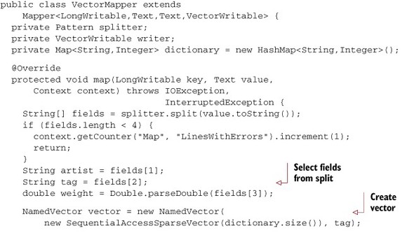
12.2.3. Converting Last.fm tags into Vectors with musicians as features
Using the dictionary generated in the previous section, we create vectors of tags so that they can be clustered together. The vectorization process is a simple MapReduce job. The Mapper selects the integer feature ID of an artist and creates a vector with a single feature. These partial vectors with one dimension are sent to the Reducer, which simply joins the partial Vector into a full Vector, as shown in the following listing.
Listing 12.7. Using integer ID mapping of the artist to convert tags into a vector

The SequentialAccessSparseVector class is used as the underlying format for representing the tags vector. K-means performs many sequential passes over the vector elements, and this representation is best suited to that access pattern. Using the partial vectors from the Mapper as input, the Reducer simply concatenates them into a full vector, as seen in the following listing.
Listing 12.8. Grouping partial vectors of tags and summing them up into full vectors

The VectorReducer merges the partial vectors and converts them into a full Vector. The Last.fm artist vectors are now ready. The next step is to run k-means to generate the topics.
12.2.4. Running k-means over the Last.fm data
The vectorization process generates around 98,999 unique tags from the Last.fm data set. You might want to cluster this into small clusters having about 30 tags each.
To start with, we try to create 2,000 tag clusters from k-means as follows:
bin/mahout kmeans -i mia/lastfm_vectors/
-o mia/lastfm_topics -c mia/lastfm_centroids -k 2000 -ow
-dm org.apache.mahout.common.distance.CosineDistanceMeasure
-cd 0.01 -x 20 -cl
On one machine, it may take about 30 minutes to complete the iterations. This is a CPU-bound process, so adding more worker machines in the Hadoop cluster will improve its completion time.
Once they have been output, the tag clusters can be inspected on the command line using the clusterdump utility using the following command:
bin/mahout clusterdump -s mia/lastfm_topics/clusters-16
-d mia/lastfm_dict/part-r-00000-dict -dt sequencefile -n 10
These are top artists for a given tag:
Top Terms:
        Shania Twain                  =>   1.126984126984127
        Garth Brooks                  =>   0.746031746031746
        Sara Evans                    =>  0.6031746031746031
        Lonestar                      =>  0.5238095238095238
        SHeDaisy                      => 0.47619047619047616
        Faith Hill                    =>  0.4126984126984127
        Miranda Lambert               => 0.36507936507936506
        Dixie Chicks                  => 0.36507936507936506
        Brad Paisley                  =>  0.3492063492063492
        Lee Ann Womack                =>  0.3492063492063492

Top Terms:
        Explosions in the Sky         =>   55.19047619047619
        Joe Satriani                  =>   51.19047619047619
        Apocalyptica                  =>   50.95238095238095
        Steve Vai                     =>  43.666666666666664
        Mogwai                        =>   39.57142857142857
        Godspeed You! Black Emperor   =>   32.00100000000101
        Yann Tiersen                  =>  30.857142857142858
        Pelican                       =>  20.285714285714285
        Do Make Say Think             =>  16.904761904761905
        Liquid Tension Experiment     =>   16.61904761904762

Top Terms:
        Justin Timberlake             =>   6.739130434782608
        Disturbed                     =>   0.391304347826087
        Timbaland                     => 0.34782608695652173
        Nelly Furtado                 => 0.30434782608695654
        Lustans Lakejer               =>  0.2608695652173913
        Michael Jackson               =>  0.2608695652173913
        Aaliyah                       => 0.21739130434782608
        Timbaland Magoo               => 0.21739130434782608
        Jonathan Davis                => 0.21739130434782608
        Sum 41                        => 0.21739130434782608
These tags could be stored in a database and later queried to produce suggestions for any tag.
This example demonstrated the trick of transforming a data set into a different view in order to apply clustering. Our next example is a bit more involved and works on a much larger, open data set of a popular Q & A website: Stack Overflow.
12.3. Analyzing the Stack Overflow data set
Stack Overflow (http://stackoverflow.com) is an online discussion website hosting questions and answers on a wide range of programming-related topics. Users ask and answer questions and vote for or against questions and answers. Users also earn reputation points for interacting on the website. For example, a user gets 10 points upon receiving an up vote on an answer given to a question. After accumulating enough points, users earn additional abilities on the site.
Thanks to Stack Overflow, all data on the website is freely available for noncommercial research. We explore Stack Overflow as a data set, and consider some of the interesting problems that can be modeled as clustering: for example, clustering questions to find related questions, clustering users to find related users, and clustering similar answers to make the answers more readable.
12.3.1. Parsing the Stack Overflow data set
The entire data sets of the stackoverflow.com site and its sister sites (superuser.com, serverflow.com, and so on), known as Stack Exchange, are available as a single file at http://blog.stackoverflow.com/category/cc-wiki-dump. The data sets are around 3.5 GB, compressed. All the data sets are similar in nature, with Stack Overflow being the largest and most prominent of the group. Uncompressed, the Stack Overflow data set is around 5 GB, split across multiple XML files. There are separate files for posts, comments, users, votes, and badges.
Parsing XML files can be tricky, especially in a Hadoop MapReduce job. Mahout provides org.apache.mahout.classifier.bayes.XMLInputFormat for reading an XML file in a MapReduce job. It correctly detects each repeated block of XML and passes it to the Mapper as an input record. This string will have to be further parsed as XML using any XML parsing library.
The XMLInputFormat class needs the starting and ending tokens of the XML block. This is achieved by setting the following keys in the Hadoop Configuration object:
...
conf.set("xmlinput.start", "<row Id=");
conf.set("xmlinput.end", " />");
...
conf.setInputFormat(XmlInputFormat.class);
...
In the Mapper, set the key as LongWritable and the value as Text, and read the entire XML block as Text in the value, including the start and end.
12.3.2. Finding clustering problems in Stack Overflow
The Stack Overflow data set contains a table of users, a table of questions, and a table of answers. There are relations between them, based on the user-id, question-id, and answer-id fields that will help you to sift and transform the data in whichever way you’d like. There are some interesting clustering problems for this data.
Clustering Posts Data for Surfacing Related Questions
It’s useful to identify questions that concern similar topics. Users browsing a post that doesn’t quite address their question might find a better answer among a list of related questions. This process of finding similar questions will be like finding similar articles in the Reuters data set. These posts are smaller than Reuters articles but larger than Twitter tweets, so TF-IDF weighting ought to give good features. It’s always good to remove high-frequency words from the data set, so keep the maximum document frequency threshold at 70 percent or even lower.
One big challenge you’ll encounter while vectorizing this data set is the lack of good tokenization of the Stack Overflow questions. Many questions and answers have snippets of code from different programming languages, and the default StandardAnalyzer isn’t designed to work on such data. You’ll have to write a parser that takes care of braces and arrays in code and other quirks in different programming languages.
Instead of using just the question, you can bundle together both questions and their answers, as well as comments, to produce larger documents and get more features to cluster similar questions. Unlike Twitter, the spelling mistakes should not harm the quality very much due to the larger size of the content. But adding a DoubleMetaphone filter would give a slight improvement in quality. Because there is lot of data, both k-means and fuzzy k-means should yield similar results. A better improvement in quality will only come by using LDA topics as features, but the CPU consumed by LDA may be prohibitively high for this data set.
Clustering User Data for Surfacing Similar Users
Imagine you’re a developer who extensively uses the Java Messaging Service (JMS) API. It might be useful to discover people who work with JMS as well. Helping users form such communities not only improves the user experience on the website, but also drives user engagement. Again, clustering can help compute such possible communities.
For clustering users, you need a vector from the features of the user. This could be the kind of content the users posts or answers, or the kind of interaction the user has with other users. These are some of the features of the vector:
- The contents of the questions or answers the user created, which includes the n-grams from text and code snippets
- The other users who replied or commented on the post the user created and interacted on.
Clustering users could be done using just the post content, by using just the common interaction counts, or both. Previously, when clustering tweets, only the content was used. It would be a good exercise to experiment on using the interaction features to cluster users.
In this model, a user is a document and its features are the IDs of other users who that user interacted with; the feature value corresponds to how much other users interacted with them. This can be weighted. For example, if user 2 commented on user 1’s post, this might map to a weight of 10. But if user 2 voted on user 1’s post, it might just be weighted a 2. If the vote was negative, it might receive a weight of –10 to indicate that these two users have a lower probability of wanting to interact with each other. Think of all possible interactions and assign weights to them. The weight of the feature user 2 in the vector of user 1 would be the cumulative weight of the interaction they have had. With these vectors and features, try clustering users based on their interaction patterns and see how it works out.
12.4. Summary
In this chapter, we examined real-world clustering by analyzing three data sets: Twitter, Last.fm, and Stack Overflow.
We started with the analysis of tweets by trying to cluster users who tweet alike. We preprocessed the data, converted it to vectors, and used it to successfully cluster users by their similarity in tweets. Mahout was able to scale easily to a data set of 10 million tweets due to the MapReduce-based implementations.
We took a small subset of a data set based on Last.fm tags and tried to generate a tag-suggestion feature for the site. We modeled the problem as a bipartite network of music artists on one part and user-generated tags on the other, with the edge weights being the number of times they co-occurred together. We clustered based on tags as well. Using this output, it was easy to generate the tag-suggestion functionality.
Finally, we examined data from Stack Overflow. We discussed solving several real-life problems on such a discussion forum using only clustering.
This concludes our coverage of clustering algorithms in Mahout. This was a gentle introduction to one aspect of machine learning, which started with the basic structures and mathematics and progressed to solving large-scale problems on a Hadoop cluster.
Now we’ll move on to discuss classification with Mahout, which entails more complex machine learning theory and some solid optimization techniques—both distributed and non-distributed—to achieve state-of-the-art classification accuracy and performance.