CHAPTER 4

Hypothesis Testing

A hypothesis is a statement about a phenomenon, trying to explain a population parameter or effect of a process when we have limited information about that population or process. A representative sample is used for observation and testing. An inference then made about the population, based on the test results. Increasing productivity after implementing a new benefits plan, treatment effect of a new medication, environmental ramifications of a chemical production plant, and using new technologies for learning, are examples where we state a hypothesis about population or process based on limited observations. Hypothesis testing is a process of statement, determining decision criteria, data collection and computing statistics, and finally making an inference. An example of the effect of a training program for customer service agents at a helpdesk can well explain hypothesis testing process. After each call, customers receive a short survey to rate the service on four criteria using a scale of one (extremely dissatisfied) to five (extremely satisfied). The criteria include timeliness of the service, courtesy of the agent, level of information offered to the customer, and overall satisfaction about the service. Total scores of a survey vary between minimum possible score of four, and maximum of 20. We will understand the results of this new training program by comparing the mean customer rating of agents who did go through the training, with those who have not yet started the program. This will be a test of independent samples. Another way of testing the effect of training program is to compare customer ratings before and after the training for the same group of employees. This will be a Z test for two samples we will explain later.

Hypothesis Testing Process

The following steps will state and test our hypothesis testing process:

Step 1. Hypothesis statement: we always state two hypotheses for each experiment. Alternative hypothesis (H_a) explains our understanding of the existing difference, or a difference created due to effect of a treatment. In case of training program, we expect the mean of customer satisfaction to increase after training. Null hypothesis (H₀) on the other hand is a negation of alternative hypothesis. H₀ is always about no difference of the population statistic before and after the treatment, no effect of treatment, or no relationship of variables. The formal statement of hypothesis is:

H_a: Employee training program will increase customer satisfaction. After training program mean customer rating score is higher than before the training.

H_a: μ > μ₀

H₀: Employee training program has no effect on customer satisfaction. Mean customer rating score will not be higher after training program. (It might be about the same or even lower than the mean of scores before training. Any observed difference is due to sampling error).

H₀: μ ≤ μ₀

This hypothesis statement leads to a one-tail test, since it identifies a direction of change. A hypothesis that does not refer to the direction of change needs a two-tail test. This type of hypothesis will be introduced later in this chapter.

Step 2. Criteria of decision: The average customer rating is 11.8 and standard deviation of scores is four. To compare mean scores observed after training with the current population mean, we will use the null hypothesis statement as expected sample statistics. If the null hypothesis is true, sample means must be around 11.8. Monotone increasing or decreasing values will not change the shape of the distribution, nor its spread. So if distribution of customer rating is normal, it will still be normal after the training, and standard deviation also will be the same as it was before training. We will use sample mean as decision criterion. This mean should be significantly different from the population mean to show a significant difference due to training. Assuming normal distribution and equal spread of sample and population, a probability boundary is required for the test. 95 percent confidence level is a common boundary, and is used in this example. Figure 4.1 demonstrates a normally distributed population with a shaded area in right tail, representing the upper five percent area under the curve. We call this value alpha level (α = 0.05), and shaded area is the critical region. Center of the distribution represents population mean, 11.8. Extremely high means of samples that are significantly different from the current population mean will be in critical region, the shaded area. We can find the Z-score of the 95 percent boundary from a standard normal distribution table as 1.64, or calculate it in Excel using NORM.INV( ) function:

=NORM.INV(0.95,0,1)

Figure 4.1(a) One tail (upper tail) test of mean. Sample mean is in critical region

Figure 4.1(b) One tail (upper tail) test of mean. Sample mean is not in critical region

Any Z score of sample means greater than the critical value of 1.64 indicate significant difference of the mean of that sample from the current population mean.

Similarly, when alpha level is 1 percent for a one-tail test, the Z score of the 99 percent boundary is 2.33. Any sample mean Z score larger than 2.33 indicates significant difference of the sample mean from population mean.

Step 3. Observations and sample statistics: data collection for an experiment starts after hypothesis statement and determining decision criteria. We may also have samples taken before stating the hypothesis, but sample information should not introduce bias in hypothesis statement. At this step, we summarize sample data and compute the statistics required for the test. This example is about difference of means for a normally distributed population, with known standard deviation. A Z-test can determine the location of sample statistic relative to the population statistic. Z score formula is:

In which:

= Sample mean

μ = hypothesized population mean

= Standard error of the sample

σ = standard deviation of the population

n = sample size

Step 4. Making a decision: The goal of all tests is to reject the null hypothesis. In this example the H₀ states, there is no significant difference between the mean customer satisfaction scores after training, and the current mean of rating. In our example data sample of ratings for 40 employees, the average is calculated as 13.3. Hypothesized mean and standard deviation of the population are 11.8 and 4 respectively. The Z score is calculated as:

This Z score is greater than the critical boundary Z score of 1.64. Sample mean is within the critical region and there is extremely low probability that a sample from the same population falls within this region. Based on this observation we can reject the null hypothesis and state that the training program significantly increased customer satisfaction.

Figure 4.1(a) and (b) demonstrate sample means within and out of the critical region respectively. Area under the curve beyond the sample statistic (mean) to the right tail, represent P-value of the test. This value is an indicator of the significance of this test. P-value of the test must be smaller than the critical boundary (5 percent) in order to reject the null hypothesis. Smaller p-values provide more significant support for rejecting the H₀. We can find the p-value of this test for calculated Z score of 2.37 from a standard normal distribution table, or calculate it in Excel using the following formula:

= 1- NORM.S.DIST(2.37,TRUE) = 0.008894

NORM.S.DIST( ) function calculates the cumulative probability under a standard normal distribution curve, given the Z score. The formula subtracts this value from 1, the entire area under the curve, to compute the area under the right tail, which is the P-value of this test. This number is the probability that we reject the H₀ while it is true.

Tests of Means

There are parametric and nonparametric tests of mean for two or more samples. Parametric tests are developed for parametric data, making assumptions including normal distribution of population under study. Nonparametric tests are used for both parametric and nonparametric data, and do not have the assumptions of parametric tests including normal distributions. In this section, we explain parametric tests of means for less than three samples.

Z Test for Independent Samples

The test explained through the hypothesis testing example is a Z test for independent samples. This test of means is used when the population mean and standard deviation are known, and researchers try to detect the effect of a factor on sample means. Use the data set provided in this chapter data file, “Z-test UT” worksheet. Customer ratings for 40 employees after training program are listed in range B2:B41. Enter the formulas demonstrated in cells E2, E3, and E4 of Figure 4.2 to compute the mean, Z score, and p-value of the Z test.

Figure 4.2 Computing mean, Z score, and P-value of the Z-test for an independent sample in Excel

Two-Sample Z Test

Sometimes the research involves comparing two samples with a null hypothesis of equal means. As a two-sample Z test example, we compare mean customer ratings of 40 employees before training and a sample of 40 who have already completed training. Large sample size allows us to use the sample variance as known variance in test of means. Data for two samples is in “Paired Z” worksheet of the data file. Use Excel function VAR.S( ) for computing variance of each range. Excel data analysis Toolpak includes a two-sample Z test tool. The Z test dialog box requires two data ranges and their calculated variances, as well as the hypothesized mean difference. The null hypothesis for this one-tail test states no difference between the means. We use zero as hypothesized difference of means. The default alpha level is 0.05 in this tool. We can change or use the same level. Results are available after selecting the output range and clicking OK. While critical boundary Z score of a one tail test with alpha level of 0.05 is 1.64, the test outcome shows a Z score of –5.249 and a very small P-value. This outcome indicates significant difference between the means of two samples, indicating significant difference made by training program (Figure 4.3).

Figure 4.3 Two-sample Z test in Excel

T-Test

When comparing the means of two samples and the standard deviation of population is not known we use t-test. For samples taken from a normally distributed population, t is a continuous distribution of location of sample means relative to the population mean. We use estimated standard error of the sample to substitute for unknown standard deviation of the population. t value is a substitute of Z score.

Sample variance is the ratio of sum of squared deviations from the mean (SS):

Sample variance =

Sample Standard deviation =

Standard error =

Estimate of standard error =

Computing “t” value is similar to Z score, by substituting the population standard deviation with estimated standard error of the sample:

Excel analysis Toolpak has two sample t-test tools for paired samples, as well as different assumptions of equal and unequal variances. Figure 4.4 demonstrates a t-test of two samples assuming unequal variances. We use the same data set of two customer rating samples for two groups, with and without training. When doing a test of means the null hypothesis is no difference of means, so we enter zero as hypothesized mean difference. The results show a critical t statistic value of 1.665 for one tail test. Absolute value of the calculated t statistic (–5.249) is much larger than the critical value which rejects the null hypothesis of equal means. The p-value of the one tail test is very small relative to alpha level of 0.05. In case we are not sure about the direction of changes due to effect of the factor we are testing, a two-tail test is appropriate. Excel t-test returns values for two-tail test too. Critical t value for two-tail test is 1.99, still smaller than the absolute value of the calculated t for this test.

Figure 4.4 T-test for two samples assuming unequal variances

Using R for Z-Test and T-Test

Import the data file Employee into R, store the data in a data frame named emp. Enter the complete path (summarized here). We will do Z-test and T-test on two columns of data, Rate1 and Rate2.

R package BSDA provides basic statistics and data analysis tools. Install and load the library. Test the equality of variances, the assumption of z-test and t-test:

Shapiro-Wilk test of normality shows normal distribution of Rate1 (p-value=0.43), but the small p-value of this test for Rate2 is a sign of non-normal distribution of this variable.

We need the mean of Rate1 and standard deviation of both variables for one sample Z-test:

Use these values as arguments of z-test:

For a paired t-test we will have the following outcome. The small p-value indicates the significance of difference between two ratings.

Analysis of Variance

Analysis of variance (ANOVA) is a parametric test of means based on sample data where two or more samples are involved. ANOVA is based on assumptions including independent samples, normal distribution of samples, and homogeneity of variances. We will use an example of three samples to explain this method. Three different suppliers provide material for a timing chain manufacturing shop. These chains are used in a new engine, so durability and shear strength are important factors. In a pilot test, manufacturer produced small batches of chains from each material and sampled them for shear strength test. Each sample includes 30 observations. Shear strength numbers, the pressure under which the chains broke, are listed as samples A, B, and C in ANOVA worksheet of the chapter data file.

Variable used for measurement in a study is a factor, so the factor of this study is pressure (psi). A study that involves only one factor is a single-factor study. ANOVA test for one factor is a single factor ANOVA. As a test of means, ANOVA has a null hypothesis of equal means for all samples:

H₀: μ₁ = μ₂ = μ₃

Alternative hypothesis states that sample means are different. At least one of the sample means is significantly different from the other samples.

Ha: μ_i ≠ μ_j at least for one pair of (i, j)

We can compute the variance of multiple samples in two different ways, between the samples and within the samples. The logic of ANOVA is that the variances calculated in two ways should not be significantly different if all samples belong to the same population. A significant difference between these two types of variances indicate that at least one sample mean is different from the others and does not belong to the same population. Figure 4.5 left side graph shows three samples with different means but significant overlap. These samples are assumes to belong to one hypothetical population. On the right side of this figure we can see two samples with overlap, and one sample with a very different mean. These three samples cannot belong to the same population. A vertical line shows the location of overall mean of samples. We will use this concept in computing variances.

Between the samples and within the samples variances may be close or very different. One measure that can create a single criterion of judgment is ratio of these two variances. This is F ratio:

There is an F critical value based on degrees of freedom of the two variances. F ratios greater than the F critical are sign of significant difference between sample means. We will discuss the F test after explaining the calculation of variances by an example. For simplicity, only the top five test results of each sample are included in calculations at this step. Formulas of mean squared errors between groups and within samples are as the following:

Figure 4.5 Three samples may have close means (left), or at least one of them being different (right)

Mean squares between groups =

Mean squares within samples =

n_j= sample j size

k = # of groups (1-k)

= group j mean

Y_ij = element i from group j

= Grand mean

The first step is computing the means of samples and overall mean of all observations. These values are used for calculating variances/mean squared errors.

In computing errors between samples we consider the mean of that sample as representative data of the entire sample, and calculate its deviation from the overall mean. Formulas in range H2:J2 in Figure 4.6 demonstrate this. Each observation is represented by the same value in computing mean squared errors, so these formulas are repeated for all observations in columns H, I, and J. We need to square these deviations and add them up for total sum of squared errors. Excel SUMPRODUCT function does all these calculations in one step. Formula in cell H8 in Figure 4.6 demonstrates SUMPRODUCT function and its arguments. Both arguments are the data rangeH2:J6.

Figure 4.6 Three sample test of means. Mean squared errors between groups

Degree of freedom for sum of squares deviation is 2. We have three samples and one statistic, the mean. Degree of freedom is 3–1=2. Mean squared error between the samples is calculated in cell H10 by dividing sum of squared errors by degree of freedom.

Calculating mean squared errors between samples follows a similar process by finding deviations of each observation from mean of the group. Range M2:O6 in Figure 4.7 shows computing deviations from sample means. We then use Excel SUMPRODUCT function in cell M8 to compute sum of squared deviations. We have 15 observations in these three samples and three sample means that should stay constant, so degree of freedom for sum of squared errors within samples is 12. Mean squares error is the ratio of sum of squared errors over degree of freedom. This value is in cell M10. F ratio is calculated in cell Q10 by dividing mean squared errors between samples by mean squared errors within samples. This F value is 0.16846.

Using standard F tables, we can find the F critical value. Using F tables (Figure 4.8) requires using degrees of freedom for numerator and denominator of the F ration. These degrees of freedom are 2 and 12 respectively, so we can find the critical value for given alpha level. A=0.05 has a critical F value of 3.89. Since our computed F ratio is 0.16846, a number less than the critical value, we fail to reject the null hypothesis. Sample means are considered equal. We used a small number of observations for demonstrating ANOVA process. All observations will be used in ANOVA test using Excel data analysis Toolpak.

Using Excel data analysis Toolpak for single factor ANOVA.

Data file ANOVA worksheet contains three samples, each with 30 observations. Single factor ANOVA is the first tool in data analysis Toolpak. The dialog box is simple. We need to organize samples in adjacent columns or rows and pass them to the dialog box as one range. Alpha level of 0.05 is used in this example. After clicking OK we will see the analysis output. In ANOVA table the calculated F ratio for 90 observations is 3.67 and F critical is 3.10. Since the computed F ratio is larger than critical F, we reject the null hypothesis and conclude that mean shear strengths of three samples are significantly different. The P-value is computed as 0.029 that is less than 0.05, the significance level of this test (Figure 4.9).

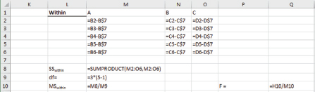
Figure 4.7 Three sample test of means. Mean squared errors within samples, and F ratio

Figure 4.8 F table

At this point, we look at the basic assumptions of ANOVA, homogeneity of variances and normal distribution of samples.

A skewed distribution is a sign of deviation from normality. Excel data analysis Toolpak can generate descriptive statistics for each data set including skewness, mean, median, maximum, and minimum. Skewness within the range of –1.96 and +1.96 and kurtosis within the range of –2 to +2, are acceptable for a normal distribution.

Cumulative distribution function (CDF) demonstrates deviations from normal distribution. Figure 4.10 shows the formulas and graph. First step is to sort observations from smallest to largest. Then compute a column of numbers where each observation of data has equal share of the percentage of observations. Selecting columns A, B, and C and creating a line graph will project values in columns B and C as lines, sharing the same vertical axis. CDF column creates a gradually increasing value, graphically a straight line, as a base of comparison for proportions of real data at each percentile. Calculations are in column C. Count of sample observations is in cell C47, which is referenced in formulas. Each cell adds the value of the cell on top of it, plus 1/30 (30 is the count of observations).

Figure 4.9 Single factor ANOVA dialog box and output

Figure 4.10 CDF plot in Excel. Projecting one data series on secondary axis

Right-click the CDF line which is almost entirely on horizontal axis due to its small values. From screen menu select “Format Data Series” to open this pane. Select “Series Options” icon and then select “Secondary Axis.” This will create a second vertical axis to the right scaled for the range of CDF data, and projects CDF line on this axis.

After projecting CDF column values on secondary axis, adjust the minimum and maximum values of primary and secondary axis to values near the range of actual data. For primary axis these limits are 1,700 and 2,300, and for secondary axis 0 and 1. Figure 4.11 shows Format Axis tool for primary axis adjustment. Double-click primary axis (left vertical axis of the chart) to open Format Axis box. Select Axis Options icon, expand Axis Options and enter values for minimum and maximum bounds. These values should contain all observations, but truncate the additional space on graph since graphs usually start from point zero. Repeat the same process for the secondary axis to limit values between 0 and 1. Points of a perfectly normal distribution will be all along the CDF line. We can observe deviations from normal, but this much of deviation does not show serious skewness. We can observe from the graph that the mean of 1996.7 (on the primary axis) is around 50th percentile of the data (on the secondary axis). In a normal distribution, about 95 percent of the data should be within +/–2 standard deviations from the mean. Calculated standard deviation of sample A is 134.38.+/–2 standard deviations from the mean is the range of 1728 to 2265. As the graph shows this range includes almost the entire data set. These observations indicate that the data set is acceptable as normal distribution.

Figure 4.11 Adjusting primary axis bounds

Homogeneity of Variance

Another assumption of ANOVA is homogeneity of variance. Based on this assumption, variances of all samples used in ANOVA should not be significantly different. There are multiple tests for homogeneity of variances, we will explain Levene test here. The null hypothesis of all tests of unequal variances is equality of variances:

Alternative hypothesis states that at least one of the variances is significantly different from others.

Levene test calculates W statistic that is F distributed. The P-value of F test less than the alpha level (usually 0.05) rejects the null hypothesis of equal variances. The formula of W is:

N = total number of observations in all samples (groups)

K = Number of samples (groups)

N_i = Sample i size

Z_i. = mean of the Z_ij for group i

Z_ij = absolute deviation of each observation from sample mean

Z_.. = mean of all absolute deviations from sample means

Leven’s formula for unequal variance test is quite similar to the formula of F ratio for ANOVA, with a difference that observations are replaced by absolute value of deviations from the mean. We do ANOVA test for deviations and the P-value of the F test will determine if the assumption of homogeneity of variances is met. Figure 4.12 shows formulas for calculating deviations from the sample means, using data file Levene worksheet. Use Single factor ANOVA from data analysis Toolpak and enter input range of E1:G31. Analysis output P-value for F test is 0.1494, which is larger than alpha level of 0.05 and fails to reject the null hypothesis of equal variances. The data meets homogeneity of variance assumption. Since sample data distributions are normal as well, ANOVA is a valid test of means.

Figure 4.12 ANOVA for absolute deviations from mean of samples. Means are in row 33

ANOVA in R

Import Chain data file into R and store values in a data frame, chain.

Gather observations in one column “gather” function needs dplyr and tidyr packages. Install these packages, load the libraries. Name the new factor column “group” and observation column “data.”

Levene test of unequal variances requires lawstat package. Install this package if not installed yet, and load the library:

Levene test results show that variances are not significantly different. If Shapio-Wilk test results show normality of the groups as well, we will do ANOVA test.

P-value of 0.0294 indicates significance of differences among mean strengths of materials.

Nonparametric Tests of Means

Z-test, t-test, and ANOVA are based on the assumption of normal distribution. ANOVA has additional assumption for homogeneity of variances. If the data is not parametric, or assumptions of each test are not met, parametric tests are not valid. We will use nonparametric tests instead. Here we explain two nonparametric tests. Mann-Whitney and signed rank Wilcoxon test are nonparametric test of means for two groups. Mann-Whitney is a test of two treatments or two independent samples. Wilcoxon is a test of paired samples, where each subject is measured twice and the outcome of each measurement is a member of one sample. Kruskal-Wallis is a nonparametric test of means for more than two groups.

Mann-Whitney and Wilcoxon test: When the two samples being compared are not normally distributed, particularly for small samples, Wilcoxon signed-rank test of means is an alternative for paired samples and Mann-Whitney test for independent samples. Both tests have similar hypotheses, but Mann-Whitney hypothesis is stated in terms of rank and Wilcoxon in terms of signed rank. Mann-Whitney states that average rank of one treatment is significantly different than the average rank of the other.

Null hypothesis for Mann-Whitney test: ranks of observations for one treatment do not tend to be systematically higher or lower than the ranks of another treatment. Two treatments do not make a difference.

Alternative hypothesis for Mann-Whitney test: ranks of observations for one treatment are systematically higher or lower than another treatment. Two treatments make a difference.

We use a subset of the customer rating data for this example to determine if training program made a significant different in customer satisfaction. 10 customer ratings were selected from each group, before and after training.

The test process requires ranking all scores from both samples. Then each observation of one sample, has lower rank than how many observations from the other sample. We can demonstrate this process as Excel worksheet formulas in Figure 4.13. Rate observations are in column B and Group labels are in column A. Data is sorted ascendingly based on values in column B, than Rank added as a sequence of incrementing number in column C. The U value in column D is obtained by an IF statement which check for group in column 1, and counts the members of the other group below it (with higher rank) through the end of the data using a conditional count function. Note the referencing of values in column A that allows us for creating this formula once in row 2 and copying it down for all values.

Sum of U values for group 1 and 2 are calculated in cells G3 and G4, using a conditional summation function. U1=83 and U2=17. Total U values is 100 which is equal to n₁n₂ (10×10). A large difference between U₁ and U₂ is a sign of significantly different ranks between the two groups. The test statistic U is the smaller of the two U values, Min(83, 17)=17 (Figure 4.13).

Mann-Whitney tables (Figure 4.14) provide critical values of U for different alpha levels. We reject the null hypothesis of no difference for U values less than the critical U. Both groups in our test have 10 observations and Nondirectional alpha level is 0.05, so the critical U value is 23. Calculated U value of the data is 17, Less than the critical value. Therefore we reject the null hypothesis and conclude that the two group means are significantly different.

Figure 4.13 Assigning Mann-Whitney U values to all observations

Figure 4.14 Mann-Whitney U table

Wilcoxon signed rank test: this test is used for evaluating difference between treatments on paired samples. For each pair, the difference of two treatments has a positive or negative sign. For example if one of the scores is before treatment and one after the treatment, higher than the score before, subtracting the initial score from after treatment will be a positive number. A lower score after treatment will generate a negative number since we are subtracting a larger number from a smaller one. Next step is ranking these differences based on their absolute value, in ascending order. Rank 1 is the smallest absolute value and highest rank is the largest absolute value of differences. We use customer ranking data from Wilcoxon worksheet of the data file for this test (Figure 4.15). To compute the ranks in Excel, add a column for absolute value of differences and use it as a reference in RANK.AVG( ) function. This function assigns average ranks for tied values. For example, absolute value of six difference scores is “1” and all need to receive the lowest rank. They all receive the average rank, (1+2+3+4+5+6)/6=3.5.

Null hypothesis of Wilcoxon test states that signs of score differences are not systematically positive or negative. Treatment does not make a difference. If this is true, positive and negative differences must be evenly mixed.

Alternative hypothesis of Wilcoxon test states that difference score signs are systematically positive or negative. There is a difference due to treatment.

After ranking differences, we will add up all ranks for positive signs together, as well as ranks for negative signs. The smaller sum of ranks is the Wilcoxon T statistic. We use Excel conditional summation SUMIF( ) function for this calculation as demonstrated in Figure 4.16, in cells I2 and I3. Positive signed ranks in our example added up to 697.5 and negative signed ranks to 122.5, so the Wilcoxon T is the minimum of the two. T = 122.5.

Figure 4.15 Signed difference score and ranks for paired samples, formula and results

Figure 4.16 Positive and negative ranks summation

Figure 4.17 Wilcoxon table of critical values

This is a one-tail test since we expect the scores to be higher after training. In Wilcoxon table of critical values (Figure 4.17), we find the critical value of 286 for a one-tail test, sample size 40, and alpha level of 5 percent. Our sample T is 122.5, smaller than the critical value. Therefore, we reject the null hypothesis of signs being evenly mixed, and conclude that customer ratings significantly increased after training.

Wilcoxon Test in R

Use “emp” data frame for Wilcoxon test.

Figure 4.18 Rank orders for three samples

Kruskal-Wallis test: This nonparametric test is used for comparing means of more than two groups. This is an alternative test for single-factor ANOVA that does not require numerical factors as long as we are able to rank sample observations, similar to Mann-Whitney test but without the limitation of only two groups. Kruskal-Wallis test compares three or more independent samples or results of different treatments. Data used for Kruskal-Wallis test must be ordinal. Original data may be ordinal, or the ranks of all observations used as ordinal data for this test. We will use the three samples of timing chain shear strength for this example. Figure 4.18 shows formulas for ranking these three samples. Each number is compared to the entire set of all three samples. Average ranking used for ties and ranks are in ascending order.

Each group will have a total rank score or T value. This value is used for comparing groups.

Null hypothesis of Kruskal-Wallis test states that ranks do not tend to be systematically higher or lower than other groups or treatments. There are no differences between groups.

Alternative hypothesis of this test states that at least one treatment is different than the others, so its ranks are systematically higher or lower than the other groups.

Kruskal-Wallis test has a distribution that approximates by χ² (Chi-Square). This test is used for goodness of fit and proportions of a multinomial population. For example if there is no difference among the shear strengths of chains from three different materials and sample sizes are equal, observed frequency of each material is 1/3. Expected frequency of failures under pressure below 2,000 psi also must be 1/3 for each group. Any significant deviation from that proportion shows a difference between materials. χ² test formula is:

In which:

f_i = observed frequency of category i

e_i = expected frequency of category i

K = number of categories

We use Kruskal-Wallis H statistic in χ² standard tables, given the degree of freedom for the data.

H values greater than critical value reject the null hypothesis of no difference among groups, and supports the hypothesis that states there are significant deviations from expected observations.

H statistic for Kruskal-Wallis is computed by the following formula:

N = Total observations in all samples

n_j = Sample size of group j

g = number of groups

T_j = Total ranks in group j

In case of a rank order test the logic of χ² is that with no difference among the groups, ranks must be distributed through the data, proportional to sample sizes. A significant deviation from proportions will cause a concentration of ranks in one direction. Degree of freedom is defined by number of groups minus one, so for three groups degree of freedom is 3–1=2. Figure 4.19 shows Excel formulas for calculating H statistic of the test. Formulas in row 2 calculate total ranks for each sample. Formula in cell J3 references these values to calculate H=6.24.

Figure 4.19 χ² Distribution table

IB

Using χ² distribution table and degree of freedom 2, the computed critical value of 6.24 is greater than 5.991, but not from the next level critical value, 7.378. At alpha level 0.05 this result indicates significant difference among the samples. At least one of the samples is significantly different from the others (Figure 4.19).

R Solution for Kruskal-Wallis Test

Use chain_g data frame to do nonparametric test of means, Kruskal-Wallis. A very small p-value demonstrates the significance of differences among means of observations for groups A, B, and C.