
Logistic regression is a method of estimating the probability of an outcome for binary categorical variables. The variable of interest is often an event. The occurrence of this event is considered “success,” and otherwise “failure.” Examples include insurance claims being a fraud or legitimate, sales quote sent to a customer being successful or not, job applications succeed or not, and if age is a factor in tendency to buy a product or service. A simple example of one predictor for the outcome is a binary dependent variable and a continuous predictor. Similar to multiple linear regression, we may have multiple predictors including categorical variables, and a nominal or ordinal response variable. The next section gives a formal development of logistic regression. If you simply want to use logistic regression, you can glance through the material to get a general idea of what logistic regression does and proceed to your software. But if you want to know why, this material shows the mathematics behind it.
Odds of Dichotomous Events
Success or failure of a sales attempt depends on a number of factors including the customer income. Using annual income as the only predictor of sales will result in a model with one continuous variable and one categorical, dichotomous response. The sales attempt is either successful or fails, so we have only two possible outcomes. A linear regression model will have unrealistic results as it will have estimations of the response variable between the two possible values of success and failure. If values of one and zero assigned to the two levels of success and failure, a linear fit line also generates values beyond these two levels that are not meaningful. A transformation of probabilities based on observed frequencies of outcomes can lead to a logistic regression solution. We will assign zero and one as two levels of response variable, zero representing the “failure” outcome and “one” the success, as in Figure 7.1.

Figure 7.1 Linear fit
Probability of success in a binomial test is a conditional probability in which the value of dependent variable (yi) is estimated based on the given values of a set of predictors (xi). We can use the notation of P(Y=yi|x1,…,xn), given that Yi is the desired outcome, or one. Probability of success is calculated based on the relative frequency of this outcome among all observations:
PSuccess = P(Y = 1) = (observed number of successes)/(Total trials)
Since the total probability space for success and failure is one:
PFailure = 1–PSuccess
Odds of these events are calculated as the following. For simplicity we call probability of success “P(x):”

These equations are best represented by a sigmoid curve that estimates the odds of outcomes (Figure 7.2).

Figure 7.2 Sigmoid curve fit for likelihood
Log Transformation of Odds
A logarithmic transformation of odds function creates a linear model:
![]()
This linear model is represented in a general form of a linear function of one or more predictors, called Logit:
Ln(OddsSuccess) = Ln(O(X)) = Ln(O(X)) = β0 + β1x1 +...+ βnxn
Solve the equation of “odds of success” for P(x):

Since Ln(O(X)) = β0 + β1x1 +...+ βnxn, then O(X) = ![]()
Replace the value of O(x) in P(x) function:
![]()
For a set of given x1,…,xn values the conditional probability of the set of given outcomes is given by the multiplication of all existing events, which are all probabilities of success, and all probabilities of failure. This product is called the likelihood function (L). The likelihood function must be maximized in order to find the optimum set of coefficients that generate the best fit to the data:
![]()
We can then transform the equation as follows:
![]()
Log Likelihood Function
Taking the natural logarithm of both sides of the likelihood equation will generate the log-likelihood function. We will maximize this function instead of the likelihood function. Logarithm is a monotonic function. Increasing values of a variable will generate increasing logarithms of those values and decreasing values of the original data will result in decreasing values of logarithms. Finding the maximum value of a log-transformed data will match the maximum point of the original data. Maximizing the values of the log-likelihood function requires the same coefficients of the variables as the original values.

A simple form of this equation for one predictor is:
![]()
Ln(A) – Ln(B)=Ln(A/B). We apply this rule to the subtraction of natural logarithms and summarize the last term by multiplying the numerator and denominator by ![]() The log likelihood function will summarize further to the following:
The log likelihood function will summarize further to the following:
![]()
Based on the natural logarithm definition we have ![]() = β0 + β1x which leads to the following steps:
= β0 + β1x which leads to the following steps:

Similarly, we can expand this equation for multiple predictors as the following:
![]()
Maximizing the log-likelihood function requires optimal coefficients of a simple or multiple logistic regression. We will use Excel solver for optimization of coefficients to demonstrate all steps of the solution.
Simple and Multiple Logistic Regression
Sale file demonstrates 200 records of calls made through a sales promotion to a customer list. The response variable Sale is the outcome of the call. Successful calls where the customer agreed to buy the product are marked “1” and otherwise “0.” Independent variables in this file are “Income,” showing the annual household income in thousands of dollars, “Household” showing the number of household residents, and “Call” showing the call duration in seconds. The manager’s understanding is that customers with higher income, having a larger number of household residents, and staying longer on phone are more likely to eventually buy the product. Our objective is to determine the optimal coefficients of a logit function that will maximize the log likelihood of success, “Sale.”
For a simple logistic regression, we will consider only “Income” as the predictor of “Sale.” Cells H1 and H2 in the Excel worksheet are reserved for decision variables of maximization, the constant value and coefficient of predictor in likelihood function (L). Two small values entered as initial numbers to start the optimization.
Log-Likelihood formula for the first row of data is entered in cell C2:
![]()
Excel formula is as follows. All references to decision variables (H1 and H2) must be absolute since we will copy this formula down in column C for all observations:
=A2*($H$1+$H$2*B2)-LN(1+EXP($H$1+$H$2*B2))
Figure 7.3 shows how this looks in Excel.
Calculate the sum of all numbers of column C in cell C203:=SUM(C2:C201)
This value is the total likelihood of all outcomes, the value we try to maximize by changing decision variables in cells H1 and H2. Start values of both decision variables are 0.001. Use the Excel solver tool for this optimization. Objective cell is the total log-likelihood, cell C203 and changing cells are H1 and H2. Solving method is generalized reduced gradient (GRG) as it is a method capable of solving nonlinear problems. Remove the default check on “Make Unconstrained Variables Non-Negative” and click on “Solve.” Solver results screen appears with “Keep Solver Solution” checked. Click on OK to keep the values (Figure 7.4).

Figure 7.3 Excel worksheet for simple logistic regression

Figure 7.4 Solver input interface, the results screen, and optimized values for β0 and β1
The logistic equation will be: Ln(O(X)) = β0 + β1x1 or O(X) = ![]()
For example the odds of purchasing for a household with annual $60,000 income will be:
O(X)= e-3.4678 + 0.0358789(60) = 0.2684
![]()
Calculating R2 and Predictor Coefficient Significance
Goodness of fit tests are necessary for statistical tests including the logistic regression model. R2 in linear regression models determines the extent in which variations of dependent variable are explained by variations of the independent variable. For a binary logistic regression model R2 is calculated by the following formula:
![]()
MLn(L)Model = Maximum Log-Likelihood of the model with all parameters
MLn(L)Null = Maximum Log-Likelihood of the model when the predictor coefficient is zero
Tests of significance compare the models with estimated coefficients of predictors, and coefficients of zero in order to determine if the estimated coefficient as the slope of a line makes a significant difference comparing to when it is zero. A zero coefficient represents no relationship between the dependent and independent variables.
For the simple logistic regression problem of sales and income, we have already calculated MLn(L)Model. Repeating the optimization process with coefficient β1 = 0 will calculate the maximum log-likelihood without the predictor. The goal is to compare the outcome and see if adding the predictor makes a significant difference in the outcome, and how the model explains variations of the dependent variable. In case of observing a significant difference between the two models, the independent variable is a significant predictor of the response. Set the predictor coefficient value to zero in cell H2. Use Excel solver and set the changing variable cell as H1 only. This is the only change from the previous solution (see Figure 7.5).
Running the Excel solver will generate the following results:
β0 = –0.6856565
MLn(L)Null = –127.5326
Full model MLn(L)Model was previously calculated as –109.7608. Using the R2 formula:
![]()

Figure 7.5 Solver set up for null model calculating MLn(L)Null
Test of significance for predictor variable Sale, is a likelihood ratio test. This test compares the likelihoods of the full and null model in obtaining results that are not significantly different. The likelihood ratio is calculated by the following formula:
![]()
The likelihood ratio for the current problem is calculated as: –2(–127.5326)+2(–109.7608)=35.54
The likelihood ratio distribution is close to χ2 so a χ2 test can determine the significance of the parameter elimination of this model. If the null and original models do not make a significant difference, the parameter is not a good predictor of the outcome. Degrees of freedom for the χ2 test equals the number of parameters eliminated from the model. Here it is one. An Excel function can directly calculate the p-value of this χ2 test:
P = CHISQ.DIST.RT(Likelihood_Ratio, 1) = CHISQ.DIST.RT(35.54, 1) = 2.49E– 09
This small p-value indicates that Income is a significant predictor of sales.
Misclassification Rate
In a copy of the worksheet calculate the estimated probability of success (Sale) for each given income ![]() . Excel formula for the first row in column H is: =1/(1+EXP(–$G$1 – B2*$G$2)). Copying this formula in column H as demonstrated in Figure 7.5 calculates probabilities for all observations. Any probability smaller than 0.5 is assigned to failure (0) and otherwise success (1). Excel logical function IF can be used to do this in column I:
. Excel formula for the first row in column H is: =1/(1+EXP(–$G$1 – B2*$G$2)). Copying this formula in column H as demonstrated in Figure 7.5 calculates probabilities for all observations. Any probability smaller than 0.5 is assigned to failure (0) and otherwise success (1). Excel logical function IF can be used to do this in column I:
=IF(H2<0.5, 0, 1)
We can also calculate the correct and misclassification rates. If an observation is “0” or “1” and estimated correctly, we can assign “1” to this outcome and if the classification is wrong comparing to the observed outcome, “0.” Use Excel function IF and logical arguments to compare values in column J by the following formula for the first row and copy for all observations:

Figure 7.6 Correct and misclassification rates
=IF(OR(AND(A2=0, H2<0.5), AND(A2=1, H2>=0.5)),1,0)
The sum of all numbers in this column represents the number of correct classifications. The correct classification rate is the ratio of this number to 200, the number of observations. The misclassification rate is the complement of this rate. Correct classification is calculated by this formula: =SUM(J2:J201)/200 =0.705 and misclassification rate is 1–0.705 =0.295 (Figure 7.6).
Multiple Logistic Regression
Multiple logistic regression solution follows a similar method as simple regression. There are a few differences because of the number of variables exist in the model. In the data worksheet reserve four decision variables for the constant and three coefficients of predictors as demonstrated in Figure 7.6. Using the Sales file with all three predictors, the general formula of Log-Likelihood is:
![]()
We can implement this formula in Excel for the first row of observations as:
Ln(L)=A6*($B$1+$B$2*B6+$B$3*C6+$B$4*D6) – LN(1+EXP ($B$1+$B$2*B6+$B$3*C6+$B$4*D6))
After copying this formula into column E for all observations and summation of log likelihoods in cell H1 we can start Excel Solver. Initial values of decision variables are 0.001. Solver solution method is GRG (Figure 7.7).
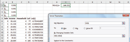
Figure 7.7 Worksheet and solver set up for multiple logistic regression
Optimum coefficients are calculated as: β0 = –4.47, β1 = 0.035, β2 = 0.2434, β3 = –0.00018
For example the probability of a household with annual income of $60,000, five residents, and staying on promotion call for 100 seconds is calculated based by the following formula:

After determining the coefficients of predictors we set the values of all predictor coefficients to zero in order to run the Solver and obtain the value of MLn(L)Null. This is one of the components of R2. Excel Solver changing cell will be “B1” only. This value is calculated using the following formula:
![]()
The significance of each variable in this model is tested by a similar method as the simple logistic regression. The decision variable (coefficient) for that variable is set to zero in a Solver run, and then a χ2 test on the likelihood ratio will determine the significance of the variable. For example the setup for testing the significance of Income is as demonstrated in Figure 7.8.

Figure 7.8 Solver and worksheet setup for testing the significance of income
This is a reduced model and after optimization its MLn(L) is calculated as –124.41. Maximum log-likelihood of the full model is already calculated as –107.722, so the likelihood ratio is: –2(–124.41)+ 2(–107.722)=33.3787.
The χ2 test p-value with “one” degree of freedom, the number of eliminated variables, is:
P= CHISQ.DIST.RT(33.3787, 1)= 7.58E– 09.
The conclusion is that Income is a significant predictor of Sales. Following a similar process for Household and Call, their P-values are 0.0461 and 0.96 respectively. These p-values determine that the number of household residents is also a significant predictor at alpha level of 5%, but call duration is not a significant predictor in this model. The correct and misclassification rates are calculated using the base formulas of simple logistic regression and adding the other predictors.
P(X)=1/(1+EXP(–$B$1–$B$2*B6–$B$3*C6–$B$4*D6))
Software Solution for Logistic Regression
We will demonstrate use of Rattle to obtain a logistic regression model for the data file we have been using (SaleData.csv, converted to comma separated variables for Rattle). We covered loading Rattle in Chapter 5 (Figure 5.3). We can also show how Rattle models this data. Figure 7.9 shows loading the data file (note that the Partition box needs to be unclicked, and then the Execute button clicked on):

Figure 7.9 Loading SaleData.csv in Rattle
Here we want the dependent variable to be Sale, which is a 0/1 variable (sale or not). There are three independent variables (Income, Household, and Call, described earlier). We can now click on the Model tab, yielding Figure 7.10 showing the Rattle modeling screen.
Given that the dependent variable is 0/1, Rattle will assume you want a logistic regression model. The model is run by clicking on the Execute button on the top row of Figure 7.10, yielding the multiple regression output in Figure 7.11.
Thus logistic regression can be supported by multiple softwares. Rattle is far easier to run than the manipulations needed in Excel. But this chapter has provided mathematical presentation of logistic regression for those students interested in knowing why it works.
Summary
Logistic regression is a highly useful tool when the dependent variable is dichotomous (either/or; yes/no; 0–1). It is a linear regression, but over data that is transformed to a nonlinear function. This is a very important tool in data mining, where many applications involve classification of cases, to include fraud detection in insurance, prediction of bank loan default, or customer profiling in marketing, with the intent of identifying potential customer profiles worth sending expensive promotional materials. It can be extended to more than two outcomes as well, as in human resources classification of employees, or refinements of any of the dichotomous cases cited earlier.

Figure 7.10 Rattle logistic regression modeling screen
This chapter has shown how logistic regression can be accomplished on Excel. There are many other software products that provide this support as well, to include R and R’s interface open source software Rattle.

Figure 7.11 Rattle multiple logistic regression model output