CHAPTER 6

Multiple Regression

Regression models allow you to include as many independent variables as you want. In traditional regression analysis, there are good reasons to limit the number of variables. The spirit of exploratory data mining, however, encourages examining a large number of independent variables. Here we are presenting very small models for demonstration purposes. In data mining applications, the assumption is that you have very many observations, so that there is no technical limit on the number of independent variables.

Data Series

In Chapter 5 we covered simple regressions, using only time as an independent variable. Often we want to use more than one independent variable. Multiple ordinary least squares (OLS) regression allows consideration of other variables that might explain changes in what we are trying to predict. Here we will try to predict the Hang Sheng Shanghai (HIS) stock index, a major Chinese trading market. We consider five additional variables, with the intent of demonstrating multiple regression, not with the aim of completely explaining change in HSI. The variables we include the S&P 500 index of blue chip stocks in the United States, the New York Stock Exchange (NYSE) index of all stocks traded on that exchange, both reflecting U.S. capital performance, a possible surrogate for the U.S. economy, which has been closely tied to the Chinese economy over the time period considered. Eurostoxx is an index of European stocks, another Chinese trade partner. Each of these three stock indexes were obtained from http://finance.yahoo.com. Brent is the price of Brent crude oil, obtained from www.tradingeconomics.com/commodity/brent-crude-oil, reflecting a cost of doing business for Chinese industry as well as for the rest of the world. Brent crude oil price can be viewed as a reflection of risk, as its price is a key component of many costs, and this price has experienced radical changes. The last variable considered is the price of gold, which can be viewed as a measure of investor uncertainty (when things are viewed as really bad, investors often flee to gold). The gold data were obtained from http://goldprice.org/gold-price-history/html. All data used was monthly for the period January 2001 through April 2016.

We model the monthly price of the HangSeng index. Monthly data for the period January 1992 through December 2017 for six potential explanatory variables (NYSE index; S&P 500 index; T Rowe Price Euro index; Brent crude oil price; price of gold; time). A regression using all six variables yielded the time series regression shown in Table 6.1.

It can be seen from Table 6.1 that time has explained nearly 90 percent of the change in the index value. However, the series is quite volatile. This regression model is plotted against the MSCI in Figure 6.1, showing this volatility.

Many of the variables included probably don’t contribute much, while others contribute a lot. An initial indicator is the p-value for each independent variable, shown in Table 6.1. P-values give an estimate of the probability that the beta coefficient is significant, which here specifically means is not zero or opposite in sign to what the model gives. In Table 6.1 the strongest fit is with NYSA and Gold, although S&P and Time also have highly significant beta coefficients. Note the 0.95 confidence limit of the beta coefficients for TRowPrEuro and for Brent, which overlap zero, a demonstration of lack of significance. Table 6.2 selects these four variables in a second model.

Figure 6.1 Full model vs. actual HangSeng

Table 6.1 HangSeng monthly time series regression

This model loses some of its explanatory power (r-squared dropped from 0.894 to 0.888) but not much. (Adding an independent variable to a given set of regression independent variables must increase r-squared.) Thus we can conclude that dropping the TRowePrice Euro index and time had little to contribute. We do see that the p-values for Brent changed, now showing up as not significant. P-values are volatile and can change radically when independent variable sets are changed.

Table 6.2 Significant variable model

Even though Time was not significant in Table 6.1, it is a convenient independent variable by itself, because it is usually the only independent variable that can accurately be predicted in the future. Table 6.3 shows the output for a simple regression of the HangSeng versus only Time.

The beta coefficient given in Table 6.3 is the trend. Figure 6.2 shows this trend, as well as demonstrating why the r-squared dropped to 0.784. Note that here time is shown as highly significant (demonstrating how p-values can change across models):

Table 6.3 HangSeng regression vs. time

Figure 6.2 HangSeng time series

Correlation

Since we have multiple independent variable candidates, we need to consider first their strength of contribution to the dependent variable (Hang Sheng index), and second, overlap in information content with other independent variables. We want high correlation between Hang Sheng and the candidate independent variables. We want low correlation between independent variables. Table 6.4 provides correlations obtained from Excel.

The strongest relationship between the HangSeng index and candidate independent variables is with NYSE at 0.901, followed by Time (0.886), S&P (0.828), Gold (0.7998) and Brent (0.767). The TRowPrEuro index is lower (how low is a matter relative to the data set—here it is the weakest). Look at the r-score for Time and HangSeng (0.886). Square this and you get 0.785 (0.784 if you use the exact correlation value from Table 6.4 in Excel), which is the r-squared shown in Table 6.3. For a single independent variable regression, r-squared equals the r from correlation squared. Adding independent variables will always increase r-squared. To get a truer picture of the worth of adding independent variables to the model, adjusted R² penalizes the R² calculation for having extra independent variables.

Table 6.4 Correlations among variables

where SSE = sum of squared errors

MSR = sum of squared predicted values

TSS = SSE + MSR

n = number of observations

k = number of independent variables

Multiple Regression Models

We now need to worry about overlapping information content. The problem is multicollinearity, overlapping explanatory content of independent variables. The strongest correlation with HangSeng was with NYSE. But NYSE also has high correlations with all of the other candidate independent variables. While cutoffs are arbitrary, one rule of thumb might be to not combine independent variables that have more to do with each other than they do with the dependent variable. NYSE and time have more to do with each other than time does with HangSeng. You would expect NYSE and S&P to be highly correlated (they come from the same market), and S&P has a higher correlation with NYSE than with HangSeng. This relationship is true for all NYSE combinations. But we might be able to find sets of independent variables that fit our rule of thumb. Time and TRowPrEuro does, but TRowPrEuro had a relatively weak relationship with HangSeng. There are about six pairs of these independent variables that have less correlation with each other than each has with HangSeng. If we also require that cross-correlation of independent variables be below 0.5 (admittedly an arbitrary requirement), we eliminate Time/Brent and S&P/Gold. That leaves four pairs (we can’t identify any triplets satisfying these restrictions, although in many data sets you can).

Of the two pairs we discarded because of mutual correlations over 0.5:

We will retain the strongest of these (S&P and Brent crude oil), with regression output in Table 6.5.

The mathematical model is thus:

HangSeng = 2938.554 + 7.153 × S&P + 87.403 × Brent

The p-value for the intercept doesn’t really matter as we need an intercept in most cases. The p-values for the other two variables are all highly significant. Plotting this model vs. actual MSCI and its trend line is shown in Figure 6.3.

Table 6.5 S&P and Brent regression

Figure 6.3 Multiple regression vs. S&P and Brent

Clearly the multiple regression fits the data better than the trend. This is indicated quantitatively in the r-square (0.863) which has to be greater than the 0.784 r-squared of the simple regression vs. time. It is less than the r-squared of the full model (0.894), but the beta coefficients of this trimmed model should be much stabler than they were in the full model (the 95 percent limits for S&P on the full model were –8.122 to –2.464, while in the trimmed model they are 6.588 to 7.718, showing a reversal in sign!); Brent’s 95 percent limits were –26.675 to 15.638, overlapping zero in the full model, and are a much stabler 78.805 to 96.001 in the trimmed model).

Using the model to forecast requires knowing (or guessing at) future independent variable values. A very good feature for Time is that there is no additional error introduced in estimating future time values.

HangSeng = 6507.564 + 60.784 × Time

That is not the case for S&P or for Brent.

HangSeng = 2938.554 + 7.153 × S&P + 87.403 × Brent

Table 6.6 Forecasts

In Table 6.6 we guess at slight increases for both S&P and Brent values for the first six months of 2018, and compare forecasts for the simple time regression with the multiple regression model.

Note that we have to guess future values for S&P and Brent. If you monitor those series closely, you might have an educated guess, but there still is error that the regression model cannot measure. R-squared can only measure error over past observations. Still, it can provide a better model here, where the trend still lags a HangSeng high cycle seen in Figures 6.2 and 6.3.

Lagged Models

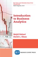
One way to avoid introducing extra error by guessing at future independent variable values is to use lags. This regresses the dependent variable against the independent variable values lagged by one or more periods. There usually is a loss of model fit, but at least there is no extra error introduced in the forecast from guessing at the independent variable values. Here we show the results of lagging S&P and Brent one, two, and three periods into the future. Table 6.7 shows the model for a lag of one period.

We can compare the three lagged models in Table 6.8 with their forecasts.

There is usually a tradeoff in lower fit (r-squared will usually drop) vs. the confidence of knowing the future independent variable values.

Table 6.7 Lag-1 model

Table 6.8 Lagged model results—S&P and Brent

Summary

Regression models have been widely used in classical modeling. They continue to be very useful in data mining environments, which differ primarily in the scale of observations and number of variables used. Classical regression (usually ordinary least squares) can be applied to continuous data. Regression can be applied by conventional software such as SAS, SPSS, or EXCEL. The more independent variables, the better the fit. But for forecasting, the more independent variables, the more things that need to be identified (guessed at), adding to unmeasured error in the forecast.

There are many refinements to regression that can be accessed, such as stepwise linear regression. Stepwise regression uses partial correlations to select entering independent variables iteratively, providing some degree of automatic machine development of a regression model. Stepwise regression has its proponents and opponents, but is a form of machine learning.