CHAPTER 5

Linear Regression

Forecasting time series is an important tool in quantitative business analysis. This chapter is primarily about linear regression. We begin with simple regression, meaning one independent variable. This is very often useful in time series analysis, with Time as the independent variable. Our focus is on linear regression, but we will compare with moving average because it is a simple approach that often does better than linear regression if seasonality or cyclical components are present in the data. Regression is a basic statistical tool. In data mining, it is one of the basic tools for analysis, used in classification applications through logistic regression and discriminant analysis, as well as prediction of continuous data through ordinary least squares (OLS) and other forms. As such, regression is often taught in one (or more) three-hour courses. We cannot hope to cover all of the basics of regression. However, we here present ways in which regression is used within the context of data mining.

Time Series Forecasting

The data set we will use for demonstration in this chapter is the percent change in real gross domestic product of the United States, measured in billions of dollars adjusted to 2009 to account for inflation. The data is quarterly, which the Federal Reserve has seasonally adjusted. The source is www.bea.gov/national/pdf/nipaguid.pdf, which at the time we downloaded provided quarterly data from 1st quarter 1947 through 1st quarter 2018 (observation 284).

Moving Average Models

The idea behind moving average models is quite simply to take the n last observations and divide by n to obtain a forecast. This can and has been modified to weight various components, but our purpose is to simply demonstrate how it works. Table 5.1 shows the last five quarterly observations, which is then used to generate two-period, three-period, and four-period forecasts.

Table 5.1 Moving average forecasts—U.S. GDP

Quarter	Time	GDP		2pd	3pd	4pd
I 2017	293	16903.24
II 2017	294	17031.09
III 2017	295	17163.89
IV 2017	296	17286.5
I 2018	297	17371.85
II 2018	298			17329.18	17274.08	17213.33

In Table 5.1, the two period moving average is simply the average of the prior two observations, or 17286.5 and 17371.85. Three and four period moving averages extend these one additional period back. These outcomes have the feature that for relatively volatile time series, the closer to the present you are, the more accurate the forecast. Moving average has the advantage of being quick and easy. As a forecast, it only extends one period into the future, which is a limitation. If there was a seasonal cycle, the 12-period moving average might be a very good forecast. But the GDP data set provided is already seasonally adjusted.

There are lots of error metrics for time series forecasts. We will use mean squared error (MSE) (to compare with regression output from Excel). This goes back to the beginning of the time series, makes two, three, and four period moving averages, squares the difference between observed and forecasted over all past observations, and averages these squared differences. For the two-period moving average this MSE was 13,740, for the three-period moving average 22,553, and for the four-period moving average 33,288.

Regression Models

Regression is used on a variety of data types. If data is time series, output from regression models is often used for forecasting. Regression can be used to build predictive models for other types of data. Regression can be applied in a number of different forms. The class of regression models is a major class of tools available to support the Modeling phase of the data mining process.

Probably the most widely used data mining algorithms are data fitting, in the sense of regression. Regression is a fundamental tool for statistical analysis to characterize relationships between a dependent variable and one or more independent variables. Regression models can be used for many purposes, to include explanation and prediction. Linear and logistic regression models are both primary tools in most general purpose data mining software. Nonlinear data can sometimes be transformed into useful linear data and analyzed with linear regression. Some special forms of nonlinear regression also exist.

OLS regression is a model of the form:

Y = β₀ + β₁ X₁ + β₂ X₂ + ... + β_n X_n + ε

where Y is the dependent variable (the one being forecast),

X_n are the n independent (explanatory) variables,
β₀ is the intercept term,
β_n are the n coefficients for the independent variables,

ε is the error term.

OLS regression is the straight line (with intercept and slope coefficients β_n) which minimizes the sum of squared error (SSE) terms ε_i over all i observations. The idea is that you look at past data to determine the β coefficients which worked best. The model gives you the most likely future value of the dependent variable given knowledge of the X_n for future observations. This approach assumes a linear relationship, and error terms that are normally distributed around zero without patterns. While these assumptions are often unrealistic, regression is highly attractive because of the existence of widely available computer packages as well as highly developed statistical theory. Statistical packages provide the probability that estimated parameters differ from zero.

Excel offers a variety of useful business analytic tools through the Data Analysis Toolpak add-in. Many students have used this suite of analytic tools before, but for those who have not, getting started has often proved challenging. We thus append a walk-through of adding this feature to your Excel software.

We can apply regression to the problem of extending a trend line. We will use the quarterly GDP data to demonstrate. The dependent variable (Y) is the quarterly GDP over the period I 1947 through I 2018. The independent variable (X) is time, an index of weeks beginning with one and ending at 285, the last available observation. Figure 5.1 displays this data.

This data is a little erratic, and notably nonlinear. OLS regression fits this data with the straight line that minimizes the SSE terms. Given the data’s nonlinearity, we don’t expect a very good fit, but the OLS model does show average trend. Here the model is:

Y = β₀ + β₁ X+ ε

where Y is Requests and X is the quarter with 1 being I 1947:

The regression output from Excel for our data is shown in Table 5.2.

This output provides a great deal of information. We will discuss regression statistics, which measure the fit of the model to the data, in the following. ANOVA information is an overall test of the model itself. The value for Significance F gives the probability that the model has no information about the dependent variable. Here, 4.431E-208 is practically zero (move the decimal place 28 digits to the left, resulting in a lot of zeros). MS for the Residual is the MSE, which can be compared to the moving average forecasts mentioned previously. Here the value of 777223.5 is worse than any of the three moving average forecasts we calculated. Finally, at the bottom of the report, is what we were after, the regression model.

Figure 5.1 Graph of GDP data

Table 5.2 Regression output for GDP time series

GDP = 15.132 + 56.080 × Time

Where Time = 1st quarter 1947, and Time = 286 Quarter II 2–18. This enables us to predict GDP in billions of dollars into the future. It is tempting to extrapolate this model far into the future, which violates the assumptions of regression model. But extrapolation is the model’s purpose in prediction. The analyst needs to realize that the model error is expected to grow the farther the model is projected beyond the data set upon which it was built. To forecast, multiply the time index by 56.080 and add 15.132. The forecasts for quarters 286 through 289 are given in Table 5.3.

Table 5.3 Time series forecasts of GDP

Quarter	GDP$2009	Time	Regression	2pdMA	3pdMA	4pdMA
2018-04-01	17371.854	286	16054	17329	17274	17213
2018-07-01		287	16110	NA	NA	NA
2018-10-01		288	16166	NA	NA	NA
2019-01-01		289	16222	NA	NA	NA

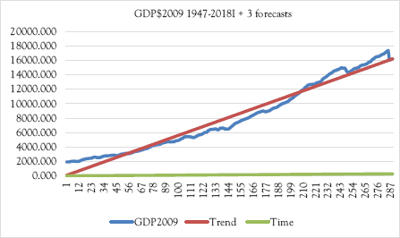
Figure 5.2 Graph of time series model

The graphical picture of this model is given in Figure 5.2.

Clearly this OLS forecast is way off. It predicts GDP in 2018I to be 16,054, when the actual is 17,372. Moving average is much closer, but moving average is very close-sighted, and can’t be extended into the future like regression models can.

Time Series Error Metrics

The classical tests of regression models are based on the assumption that errors are normally distributed around the mean, with no patterns. The basis of regression accuracy are the residuals, or difference between prediction and observed values. Residuals are then extended to a general measure of regression fit, R-squared.

SSE: The accuracy of any predictive or forecasting model can be assessed by calculating the SSE. In the regression we just completed, SSE is 219,954,255, an enormous number meaning very little by itself (it is a function not only of error, but of the number of observations). Each observation’s residual (error) is the difference between actual and predicted. The sign doesn’t matter, because the next step is to square each of these errors. The more accurate the model is, the lower its SSE. An SSE doesn’t mean much by itself. But it is a very good way of comparing alternative models, if there are equal opportunities for each model to have error.

R²: SSE can be used to generate more information for a particular model. The statistic R² is the ratio of variance explained by the model over total variance in the data. Total squared values (6,286,706,981 in our example) is explained squared dependent variable values (6,066,752,726 in our example) plus SSE (219,954,255 in our example). To obtain R², square the deviation of predicted or forecast values from the mean of the dependent variable values, add them up (yielding MSR), and divide MSR by (MSR + SSE). This gives the ratio of change in the dependent variable explained by the model (6,066,752,726/6,286,706,981 = 0.9650 in our example). R² can range from a minimum of 0 (the model tells you absolutely nothing about the dependent variable) to 1.0 (the model is perfect).

where SST is the sum of squared deviations of the dependent variable from its own mean,

SSE is the sum of squared error (difference between actual dependent variable values and predicted or forecast values).

There are basic error metrics for general time series forecasts. The regression models from Excel report SSE as we have just seen. Another way to describe SSE is to take error for each observation, square these, and sum over the entire data set. Calculating the mean of SSE provides MSE. An alternative error metric often used is mean absolute deviation (MAD), which is the same thing except that instead of squaring errors, absolute values are taken. MAD is considered more robust than MSE, in that a very large error will affect MSE much more than MAD. But both provide useful means of comparing the relative accuracy of time series, given that they compare models over exactly the same data. A more general error metric is mean absolute percentage error. Here the error for each observation is calculated as a percentage of the actual observation, and averaging over the entire time series.

Seasonality

Seasonality is a basic concept—cyclical data often has a tendency to be higher or lower than average in a given time period. For monthly data, we can identify each month’s average relative to the overall year. Here we have quarterly data, which is deseasonalized, so we expect no seasonality. But we can demonstrate how seasonality is calculated. We calculate the average by quarter from our data set for quarters I through IV over the data set (1947–1st quarter 2018). Table 5.4 shows these averages.

The calculation is trivial—using the Average function in Excel for data by quarter and the overall average for entire series. Note that there is a bit of bias because of trend, which we will consider in time series regression. Nonetheless, this data shows no seasonality, indicating that the bureau of commerce does a good job of deseasonalizing GDP.

We can include seasonality into the regression against Time by using dummy variables for each quarter (0 if that observation is not the quarter in question—one if it is). This approach requires skipping one time period’s dummy variable or else the model would be overspecified, and OLS wouldn’t work. We’ll skip quarter IV. An extract of this data is shown in Table 5.5.

Table 5.4 Seasonality indexes by month—Brent crude oil

Quarter	Average	Season Index
I	8156.630	1.001
II	8089.151	0.993
III	8145.194	1.000
IV	8195.525	1.006
Year	8146.660

Table 5.5 Seasonal regression data extract—GDP

Quarter	GDP$2009	Time	Q1	Q2	Q3
1947 I	1934.471	1	1	0	0
1947 II	1932.281	2	0	1	0
1947 III	1930.315	3	0	0	1
1947 IV	1960.705	4	0	0	0

The Excel output for this model is given in Table 5.6.

Table 5.6 Regression output for seasonal GDP

Note that R Square increased from 0.965 in Table 5.2 to 0.966. Adjusted R Square rose the same amount, as there were few variables relative to observations. Note however that while Time is significant, none of the dummy variables are. The model is now:

GDP = 7.887 + 56.080 × Time + coefficient
of dummy variable per quarter

The nice thing about this regression is that there is no error in guessing future variable values. The forecasts for 2018 are shown in Table 5.7.

The seasonal model has more content, and if there is significant seasonality can be much stronger than the trend model without seasonality. Here there is practically little difference (as we would expect, as the data was deseasonalized). Our intent here is simply to show how the method would work.

We can demonstrate error metrics with these forecasts. We limit ourselves to 1948s four quarterly observations to reduce space requirements. Table 5.8 shows calculations.

Absolute error is simply the absolute value of the difference between actual and forecast. Squared error squares this value (skipping applying the absolute function, which would be redundant). Absolute percentage error divides absolute error by actual. The metric is the mean for each of these measures. In this case, the numbers are very high as can be seen in Figure 5.2 where the trend line is far below actual observations in 1948. The actual GDP has a clear nonlinear trend.

Table 5.7 Comparative forecasts

Time	Quarter	Time regression	Seasonal regression
287	II 2018	16,054	16,052
288	III 2018	16,110	16,108
289	IV 2018	16,166	16,159
290	I 2019	16,222	16,232

Table 5.8 Error calculations

Time	Actual	Time Reg	Abs error	Squared error	% Error
5	1989.535	295.529	1694.006	2,869,656	573.2
6	2021.851	351.609	1670.242	2,789,709	475.0
7	2033.155	407.688	1625.467	2,642,142	398.7
8	2035.329	463.768	1571.561	2,469,804	338.9

Software Demonstrations

For OLS regression, Excel was demonstrated earlier. The only limitation we perceive in using Excel is that Excel regression is limited to 16 independent variables. We can also use R for linear regression.

To install R, visit https://cran.rstudio.com/

Open a folder for R

Select Download R for windows

To install Rattle:

Open the R Desktop icon (32 bit or 64 bit) and enter the following command at the R prompt. R will ask for a CRAN mirror. Choose a nearby location.

>install.packages”(rattle)”

Enter the following two commands at the R prompt. This loads the Rattle package into the library and then starts up Rattle.

>library(rattle)

>rattle()

If the RGtk2 package has yet to be installed, there will be an error popup indicating that libatk–1.0–0.dll is missing from your computer. Click on the OK and then you will be asked if you would like to install GTK+. Click OK to do so. This then downloads and installs the appropriate GTK+ libraries for your computer. After this has finished, do exit from R and restart it so that it can find the newly installed libraries.

When running Rattle a number of other packages will be downloaded and installed as needed, with Rattle asking for the user’s permission before doing so. They only need to be downloaded once.

Figure 5.3 Rattle data-loading screenshot

Figure 5.3 shows an initial screen where we load the quarterly data file:

The data file is linked in the Filename menu. When we click on Execute, we see the data types. We select Target for GDPC1 as this is what we wish to predict. Note that we deselect the partition box—if we don’t do that, Ratte will hold 30 percent of the data out for testing. While that is useful for some purposes, we don’t want to do that here. Again, click on Execute to induce R to read GDP as the target. We now want to run a linear model. Click on the Model tab, yielding Figure 5.4.

R displays its options under linear models. Using the quarterly data, we select Numeric and Linear, and click on Execute. This yields the output shown in Figure 5.5.

Summary

There are many ways to extend time series. Moving average is one of the easiest, but can’t forecast very far into the future. Regression models have been widely used in classical modeling. They continue to be very useful in data mining environments, which differ primarily in the scale of observations and number of variables used. Classical regression (usually OLS) can be applied to continuous data. Regression can be applied by conventional software such as SAS, SPSS, or EXCEL.R provides a linear model akin (but slightly different from) to OLS. There are many other forecasting methodologies, to include exponential smoothing. We covered the methods that relate to the techniques we will cover in future chapters. We have also initially explored the Brent crude oil data, demonstrating simple linear models and their output.

Figure 5.4 Linear regression screenshot

Figure 5.5 R linear model output—quarterly GDP

APPENDIX

Data Analysis Toolpak Add-In

Begin with Figure 5.6, and select File in the upper left corner.

Figure 5.6 Excel sheet

This produces Figure 5.7.

Figure 5.7 File results

Click on Options (bottom entry on menu—you get an Excel Options window—Figure 5.8). In the window, under Inactive Application Add-ins, select Analysis ToolPak.

Click on Add-ins on the left column and get Figure 5.9.

Make sure that Analysis ToolPak is selected, and click on the Go… button. That will give you the Data Analysis Tab (Figure 5.10), which includes Regression (used for both single and multiple regression) as well as correlation tools.

The Data tab is displayed in gray on the top bar in Figure 5.9—Data Analysis will be on far right on next row after you add-in. Note that this same window allows you to add-in SOLVER for linear programming.

Figure 5.8 Excel options window

Figure 5.9 Select analysis toolPak

Figure 5.10 Data analysis tab

To Run Regression

You need to prepare the data by placing all independent variables in a contiguous block before you start—it is a good idea to have labels for each column at the top. Go to Data on the top ribbon, on the window you get select Data Analysis (Figure 5.11). Select Regression (you have to scroll down the menu):

Figure 5.11 Regression windows

Enter the block for the dependent variable (X)

Enter the block for the independent variables (one or more Ys)

If you have labels, you need to click the Labels box.

You have choices of where to put the model

You obtain an OUTPUT SUMMARY (see Table 5.2 and others earlier in this chapter).

Usually it is best to place on a new worksheet, although you might want to place it on the same page you are working on.

To Run Correlation

Correlation is obtained as shown in Figure 5.12.

Figure 5.12 Select correlation

You get the window shown in Figure 5.13.

Enter the block of data (they have to be all numeric, although you can include column labels if you check the “Labels in First Row” box—highly recommended. You again have a choice of where to place the correlation matrix (a location on your current Excel sheet, or a new Excel sheet).

Figure 5.13 Correlation input window