
21
CAPITAL INVESTMENT DECISIONS
Advanced Topics
CHAPTER INTRODUCTION
In Chapter 20, we introduced key elements of capital investment decisions. In this chapter, we will cover advanced topics, including dealing with risk and uncertainty, capital budgeting and rationing, and methods of evaluating the effectiveness of the capital investment decision process. Finally, we will review best practices in presenting capital investment decisions.
DEALING WITH RISK AND UNCERTAINTY IN CAPITAL INVESTMENT DECISIONS
Since we are dealing with expectations, predictions, and projections of future performance, capital investment decisions have an inherent level of risk and uncertainty. The risk and uncertainty can be extreme in projects that extend over a long period or involve rapidly changing environmental and competitive factors (almost all markets now!).
There are two broad techniques for addressing risk and uncertainty in capital investment decisions:
- Use of an appropriate discount rate for the project risk.
- Analysis, evaluation, and flexing of financial projections.
Utilize an Appropriate Discount Rate
Many firms use a single discount rate for all capital projects. In many cases, the origin and basis of the discount rate is not known or well understood. The discount rate should be reviewed periodically, and the appropriateness of using it on a specific project should always be considered.
The starting point for selecting the discount rate should be the firm's overall cost of capital. This weighted average cost of capital (WACC) is a blend of all risk and return factors for the company. The rate for a specific project should be reviewed to determine if it is appropriate for the specific risk characteristics of that project.
Let's begin with the security market line, commonly known as the risk‐return graph. While its origin lies in the capital asset pricing model (CAPM) for financial securities, the concept transfers to real investments as well. Investors and managers can choose to invest in a wide range of investment alternatives, each with its own level of a risk. As you move down the investment risk axis, the theory holds that investors should have a higher return expectation. (See Figure 21.1.)

FIGURE 21.1 Risk and Return
The firm's weighted average cost of capital is simply one point on this curve, representing the required return for all investors in the company's debt and equity. The spectrum of potential investments for a firm ranges from low‐risk investments such as replacing equipment on the manufacturing line to investing in a high‐risk venture. Figure 21.2 illustrates typical investments a firm may evaluate; the actual placement and ranking would be very situation and project specific. Replacing the equipment on the manufacturing line would generally have low risk since the firm already has experience in this activity and there is little risk of loss since it appears to be needed to support revenue. Replacing an existing product would also likely have lower risk than the firm‐wide composite (WACC). However, investments to develop a new product, acquire a business, or develop a new technology would likely be higher than the firm's WACC.

FIGURE 21.2 Risk and Expected Return
If the firm uses the WACC to evaluate higher‐risk programs, it runs the risk of approving projects that have higher risk than expected returns. Conversely, if the WACC is used to evaluate projects with lower risk, it may reject projects that should be approved. Refer to Chapter 19 for a more complete discussion on the cost of capital and WACC.
In theory, the firm could research similar investments and develop an expected return (discount rate) for each individual project. This can be time‐consuming and difficult. Most firms would develop a practical framework that allows for some recognition of differing risk levels, as illustrated in Figure 21.3.

FIGURE 21.3 Setting Hurdle Rates Based on Risk
In this example, the firm's WACC is estimated to be 12%. The firm could establish an overall hurdle rate of 14% by tacking on a premium or cushion of 2%. For project categories with lower risks, the hurdle rate would be reduced. For investment categories with higher risks, the hurdle rate would be increased to require a higher expected return to be approved. The firm can override the hurdle rate for any specific project if that is deemed appropriate. The firm's WACC and hurdle rates are typically reviewed and updated if appropriate, on an annual basis. Any significant events that change the risk profile would also warrant reconsideration.
Analysis, Evaluation, and Flexing of Financial Projections
I have always found that understanding and evaluating the financial projections in a capital decision are among the most important and difficult aspects of the review process. For significant projects, it may be appropriate to look at several projection scenarios and analyses. The best practices in projecting and evaluating long‐term projections discussed in Chapter 14 should be employed in significant projects.
For significant projects with extended time horizons, a thorough plan and financial projection should be developed to support the capital investment decision. The following capital investment decisions would warrant a complete business plan and detailed financial projections:
- New product
- New business unit
- Acquiring a business or company
There are several tools that have proven effective in dealing with risk and uncertainty in capital investment decisions. We will build on our illustration of the new pharmaceutical development to treat procrastination.
Base Case. The base case employs a discounted cash flow (DCF) analysis using the most likely estimates for all variables. This case represents a single outcome from a range of potential outcomes and includes many assumptions about future events and performance. The base case is the project investment analysis in Table 21.1.
TABLE 21.1 Project Investment Analysis: Procrastination Pharmaceutical ![]()
| Vance Pharma Co. | Project Investment Analysis $000's (Unless otherwise noted) | |||||||||
| New Treatment for Procrastination | ||||||||||
| Incremental Changes | 2018 | 2019 | 2020 | 2021 | 2022 | 2023 | 2024 | 2025 | Terminal Value | |
| Revenues | – | – | – | 25,000 | 75,000 | 125,000 | 200,000 | 225,000 | ||
| Cost of Revenues | ||||||||||
| On Incremental Revenues | 25% | – | – | – | 6,250 | 18,750 | 31,250 | 50,000 | 56,250 | |
| Project Savings | – | |||||||||
| Incremental Cost of Revenues | – | – | – | 6,250 | 18,750 | 31,250 | 50,000 | 56,250 | ||
| Gross Margin Impact | – | – | – | 18,750 | 56,250 | 93,750 | 150,000 | 168,750 | ||
| Operating Expenses: | ||||||||||
| On Incremental Revenues | 15% | – | – | – | 3,750 | 11,250 | 18,750 | 30,000 | 33,750 | |
| Project Savings | ||||||||||
| Project Costs and Expenses | 20,000 | |||||||||
| Depreciation on Project Capital | 10,000 | 10,000 | 10,000 | 10,000 | 10,000 | |||||
| Incremental Operating Expenses | 20,000 | 10,000 | 10,000 | 13,750 | 21,250 | 28,750 | 30,000 | 33,750 | ||
| Operating Profit | −20,000 | −10,000 | −10,000 | 5,000 | 35,000 | 65,000 | 120,000 | 135,000 | ||
| Tax | 40% | 8,000 | 4,000 | 4,000 | −2,000 | −14,000 | −26,000 | −48,000 | −54,000 | |
| Operating Profit After Tax | −12,000 | −6,000 | −6,000 | 3,000 | 21,000 | 39,000 | 72,000 | 81,000 | ||
| Operating Cash Flow: | ||||||||||
| Depreciation | 10,000 | 10,000 | 10,000 | 10,000 | 10,000 | |||||
| (Inc) Dec in Accounts Receivable | – | – | −938 | −2,813 | −4,688 | −7,500 | −8,438 | |||
| (Inc) Dec in Inventories | – | −1,875 | −5,625 | −9,375 | −15,000 | −16,875 | −16,875 | |||
| Capital Expenditures | −50,000 | |||||||||
| Incremental Cash Flows | −62,000 | 4,000 | 2,125 | 6,438 | 18,813 | 29,313 | 47,625 | 55,688 | 371,250 | |
| Cumulative Cash Flows | −62,000 | −58,000 | −55,875 | −49,438 | −30,625 | −1,313 | 46,313 | 102,000 | 473,250 | |
| PV Factor | 0.870 | 0.756 | 0.658 | 0.572 | 0.497 | 0.432 | 0.376 | 0.327 | 0.284 | |
| PV Cash Flow | −53,913 | 3,025 | 1,397 | 3,681 | 9,353 | 12,673 | 17,904 | 18,204 | 105,532 | |
| NPV | $117,856 | Discount Rate | 15% | |||||||
| IRR | 37% | PH Growth Rate | 0% | |||||||
| Payback | 6 Years | |||||||||
Sensitivity Analysis. This technique determines the sensitivity of the decision criteria (e.g. NPV) to changes in the assumptions used in the base case. Table 21.2 presents the traditional sensitivity analysis, showing the base case of $117.8 and the resultant NPV values at different assumptions of revenue and development costs.
TABLE 21.2 Sensitivity Analysis ![]()
| Procrastination Pharmaceutical | ||||||
| Sensitivity Analysis | NPV | |||||
| Revenues (M) | ||||||
| 175.0 | 200.0 | 225.0 | 250.0 | 275.0 | ||
| $ 18.0 | 88.0 | 105.0 | 122.0 | 137.0 | 154.0 | |
| Development | 19.0 | 86.0 | 103.0 | 120.0 | 135.0 | 152.0 |
| Costs (M) | 20.0 | 83.0 | 101.0 | 117.8 | 133.0 | 150.0 |
| 21.0 | 81.0 | 98.0 | 115.0 | 131.0 | 149.0 | |
| 22.0 | 77.0 | 94.0 | 111.0 | 129.0 | 146.0 | |
Table 21.2 shows that this project could have a NPV as low as $77.0 million to a high of $154.0 million within the ranges of these assumptions. This provides great context to the decision makers, giving insight into the dynamics of the investment.
Breakeven Analysis.Table 21.3 presents a different form of sensitivity analysis that highlights the impact of a 10% change in each variable and determines how far the assumptions can change before resulting in a breakeven NPV value.
TABLE 21.3 Sensitivity and Breakeven Analysis ![]()
| Procrastination Pharmaceutical | |||||
| Sensitivity and Breakeven Analysis | |||||
| Key Assumptions | |||||
| Base | 10% Change | NPV | % Change in NPV | Breakeven Approx. Value NPV=0 | |
| Base | 117.9 | 117.9 | |||
| Sales (2025) | 225.0 | 202.5 | 101.8 | −13.6% | 56.5 |
| Cost & Expense Levels | 40% | 44.0% | 87.9 | −25.4% | 56.0% |
| Tax Rate | 40.0% | 44.0% | 103.3 | −12.4% | NMF |
| Initial Outlay | 70.0 | 77.0 | 114.2 | −3.1% | 250.0* |
| Terminal Value | 371.3 | 334.1 | 107.3 | −9.0% | 0 |
| Discount Rate | 15.0% | 16.5% | 93.2 | −20.9% | 30.0% |
* Dependent on assumptions capital vs. expense
Scenario Analysis. This important tool determines projected NPV of the project under specified scenarios (e.g. recession, best case, competitive reaction, etc.). Projections for each specific scenario are developed, and the investment is evaluated under each scenario.
Steps to develop scenarios:
- Select potential scenarios (e.g. general economic, price of oil, competitive reaction, adoption rates).
- Develop projections under each scenario. This is a critical aspect of scenario planning. Unlike sensitivity analysis, where we simple flex selected variables, we will revise the base projections for expected changes under the scenario. For example, in a recession, a company may experience price pressure and lower demand. That company may also expect different interest rates, labor rates, and commodity pricing.
- Measure scenario using NPV, IRR, payback, and so forth.
- Use this insight in evaluating the project.
In our example of the development of a procrastination treatment, there are several potential scenarios to consider, including:
- Product development efforts fail, and the project is abandoned.
- Product development is successful but revenues do not meet projections because a competitor introduces a similar product.
- Revenues exceed the base projections.
Others:
- Prices are controlled by government.
- A recession occurs.
The results of each of each scenario can be evaluated and presented to decision makers. (See Figure 21.4.) In addition to providing insight into all potential outcomes, an important benefit is that it encourages the identification of important checkpoints and management options. For example, an executive should insist on identifying and monitoring the key drivers that will lead to abandonment of the project. Timely determination of ultimate failure will allow the project to be terminated at the earliest possible time, resulting in minimizing the loss on the project and allowing resources to be deployed to other, more promising projects.

FIGURE 21.4 Scenario Recap 
Event, Decision, and Option Trees. Event, decision, and option trees can be very effective tools in evaluating and presenting capital investment decisions. An event tree generally refers to a presentation of alternative events or outcomes. Decision or option trees include future management decisions (options) as one or more events in the future. They build on the concept of scenario analysis described earlier. Decision and event trees are a useful way to visualize, communicate, and evaluate various scenarios, especially future projects or other decisions where the outcomes are uncertain. Projects may result in several different outcomes (success, failure, delay) and may also be subject to management decisions after the initial project approval (delay, cancel, etc.). For example, a firm may face a choice to replace an existing product with a new product or continue to sell the existing one. This is unlikely to be a single decision point. How successful will the new product be? What will happen to the sales of the existing product if not replaced? What subsequent options will management have to optimize the result? A decision tree identifies and presents decisions and probable outcomes at each stage of a project.
The simple illustration in Figure 21.5 is a very effective way to lay out various management decisions and to describe potential outcomes resulting from each alternative scenario/decision. Each of the six potential outcomes will have a probability of occurrence and an estimated value (e.g. NPV, sales, earnings per share). Each of these six outcomes will also have a second level of management options or decisions.

FIGURE 21.5 Decision Tree
Simulations. In simulations, decision criteria would be estimated across an entire probability distribution for key variables. For example, revenues, margins, investments, and other key variables would be analyzed to develop a spectrum of potential outcomes and associated probabilities. The biggest downside is the need to develop estimates and probabilities across the entire distribution of potential outcomes for each variable and then to determine value (e.g. NPV) under each combination of variables. Simulations can be used for large development projects and are typically used by large consumer product and retail companies where history is readily available to develop estimated outcomes and probabilities.
The output of a simulation would provide a range and probability distribution for a project that can give decision makers insight on the project dynamics. For many decisions, the scenario and event tree methods just described will get decision makers close to the same insight with far less effort.
Illustration: Decision Tree for Procrastination Pharmaceutical
The base case for the development and introduction of the pharmaceutical for treatment of procrastination presents a single scenario outcome for that project. It includes many assumptions about the timing and success of the development process and also assumes that management has no ability in the future to change the course of development and introduction if circumstances change. Figure 21.6 provides a simple illustration of multiple outcomes for this project. Note that this illustration is a gross oversimplification of the process for developing and obtaining approval for new pharmaceuticals!

FIGURE 21.6 Event/Option Tree
This analysis provides several additional insights. First, the base case assumes approval and a solid revenue stream resulting in an NPV of $117,856. However, there is a 30% chance that the pharmaceutical will not be approved, resulting in a negative NPV of $12,000 ($20,000 research expense less 40% tax savings). Second, it highlights that there are also additional scenarios that revenues will fall short or exceed the base case, with the shortfall resulting in a negative NPV of $2,226.
Clearly the addition of this analysis adds significant insight to the decision. The results of this analysis can be summarized in Figure 21.7, but the decision tree also has outright value in understanding and communicating the dynamics of the investment decision.

FIGURE 21.7 Option Event Summary for Procrastination Pharmaceutical
Real Options and Option Value
Real options build on the principles of option trees illustrated earlier. Essentially, the advocates of real options apply option pricing models for securities to “real” investments. While this is a fascinating area for math majors, I find it difficult to effectively utilize in most practice situations. In addition, presenting a value from a complex formula is difficult to explain and doesn't add value in terms of understanding the dynamics of an investment decision.
A related concept that is often used is the option value. An investment may have a positive (or negative) NPV based on the primary opportunity under evaluation. It may also provide a platform or ability to pursue another opportunity. For example, the procrastination treatment may also be the foundation for another treatment, for smart phone attention deficit (SPAD). Another plan and projection can be developed for this new treatment to commence after the procrastination treatment is completed. The potential NPV of this second project can be estimated and considered in the evaluation of the program (see Figure 21.8).
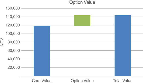
FIGURE 21.8 Option Value Illustration
The option value is often used to justify a program that has negative or marginal NPV (prospect for value creation). Of course, this can be abused if not managed properly.
PRESENTING CAPITAL INVESTMENT DECISIONS
Capital investment decisions are a critical aspect of the management process, since it is the determination of what projects should be approved to create value for shareholders. In addition to effectively developing plans and investment evaluations for significant projects, it is important that FP&A teams also develop effective presentations to management in order to facilitate the overall evaluation and approval of projects.
Many projects, for example a large developmental project or acquisition, will be accompanied by a complete business plan that supports the economic valuation and analysis described in this chapter.
Figure 21.9 provides an illustration of a recap or approval summary for a capital investment decision. The advantage of this one‐page summary is that all relevant information is presented on this single document. Of course, this recap will likely be supported by a detailed presentation and business case.

FIGURE 21.9 Capital Investment Summary
CAPITAL BUDGETING AND RATIONING
Although in theory we assume that capital is available for any investment opportunity with a positive NPV, as a practical matter firms must allocate capital and evaluate many potential projects for possible investment. This process often occurs as part of the strategic and operational planning process and product development activities. Typically, operating and business unit executives identify more potential capital projects than the company is able or willing to fund, with reasons ranging from cash or profit constraints to management capacity. Firms employ several techniques to provide insight on which projects should be selected.
Raise the Hurdle or Discount Rate. If the hurdle or discount rate were raised for all projects, some investments would no longer have positive NPV and would be rejected. However, this has the effect of penalizing all projects.
Profitability Index (PI). The PI is a tool used to measure the value of a project compared to the initial investment.
The profitability index is computed as follows:
For our drug development example, the PI is computed as follows:

The firm can then rank projects by the index and approve those projects with the highest PI as illustrated in Table 21.4. In this example, if the capital budget for the coming year must be held to $325,000, then the last five projects would not be pursued.
TABLE 21.4 Capital Investment Allocation ![]()
| Vance Pharmaceutical | ||||||
| Capital Investment Allocation | ||||||
| Overall | Profitability | Cumulative | ||||
| Rank | Project Description | Investment | NPV | IRR | Index | Investment |
| 6 | Airplane for CEO | 4,000 | 8,000 | 60.0% | 2.000 | 4,000 |
| 3 | Procrastination Drug | 70,000 | 117,856 | 0.37 | 1.684 | 74,000 |
| 11 | Replace Building 2 Equipment | 3,200 | 2,900 | 50.0% | 0.906 | 77,200 |
| 5 | Laziness Treatment | 32,000 | 22,000 | 17.0% | 0.688 | 109,200 |
| 10 | Info Technology‐Enterprise System | 12,000 | 6,100 | 15.0% | 0.508 | 121,200 |
| 7 | Automate Manufacturing | 200,000 | 96,414 | 28.0% | 0.482 | 321,200 |
| 5 | Expand Distribution Center | 4,875 | 2,265 | 18.5% | 0.465 | 326,075 |
| 8 | All Other < 1,000 | 16,000 | 4,200 | 0.17 | 0.263 | 342,075 |
| 12 | New Corporate Headquarters | 4,000 | 23 | 0.1% | 0.006 | 346,075 |
| 2 | New Roof | 1,200 | −120 | −11.0% | −0.100 | 347,275 |
| 4 | Info Technology‐Security | 7,000 | −2,100 | −7.0% | −0.300 | 354,275 |
| 1 | Wastewater Treatment | 15,000 | −5,260 | −15.0% | −0.351 | 369,275 |
| Total | 369,275 | 252,278 | 25% | 0.683 | ||
The problem with using only a financial measure to evaluate projects is that many projects have important nonfinancial attributes that must be considered, ranging from executive preferences to statutory requirements. In this case, the casualties of PI ranking would prohibit repairing the roof and addressing the wastewater issue, an apparent Environmental Protection Agency (EPA) requirement.
Holistic Approach. To reflect both the financial rankings and other important business issues, leading finance organizations develop a holistic view of all capital investments and rank them, taking into account a multitude of factors, including PI, EPS impact, strategic importance, and statutory requirements. Table 21.5 incorporates all factors in a single summary. This presentation will generally facilitate the decision around capital priorities.
TABLE 21.5 Capital Plan Ranking ![]()
| Vance Pharmaceutical | |||||||||||
| Capital Investment Allocation | |||||||||||
| Overall | Profitability | Cumulative | EPS Accretive | Strategic | Statutory | ||||||
| Rank | Project Description | Investment | NPV | IRR | Index | Investment | Year | $0.00 | Importance | Requirement | Notes |
| 1 | Wastewater Treatment | 15,000 | −5,260 | −15.0% | −0.351 | 15,000 | Low | Yes, EPA Requirement | |||
| 2 | New Roof | 1,200 | −120 | −11.0% | −0.100 | 16,200 | Leaking roof jeopardizing FDA License | ||||
| 3 | Procrastination Drug | 70,000 | 117,856 | 0.37 | 1.684 | 86,200 | 2021 | 0.11 | High | No | Most important PD effort |
| 4 | Info Technology‐Security | 7,000 | −2,100 | −7.0% | −0.300 | 93,200 | High | No, but… | Cyber threats increasing | ||
| 5 | Laziness Treatment | 32,000 | 22,000 | 17.0% | 0.688 | 125,200 | 2024 | Yes | |||
| 5 | Expand Distribution Center | 4,875 | 2,265 | 18.5% | 0.465 | 130,075 | No | Yes | Support sales growth, new products | ||
| 6 | Airplane for CEO | 4,000 | 8,000 | 60.0% | 2.000 | 134,075 | 2018 | Yes | Expense/time savings | ||
| 7 | Automate Manufacturing | 200,000 | 96,414 | 28.0% | 0.482 | 334,075 | 2020 | 0.200 | Moderate | No | |
| 8 | All Other < 1,000 | 16,000 | 4,200 | 0.17 | 0.263 | 350,075 | |||||
| 10 | Info Technology‐Enterprise System | 12,000 | 6,100 | 15.0% | 0.508 | 362,075 | No | Replace existing/add functionality | |||
| 11 | Replace Building 2 Equipment | 3,200 | 2,900 | 50.0% | 0.906 | 365,275 | 2020 | ||||
| 12 | New Corporate Headquarters | 4,000 | 23 | 0.1% | 0.006 | 369,275 | Yes | No | Image/Locate in Financial Center | ||
| Total | 369,275 | 252,278 | 25% | 0.683 | |||||||
TABLE 21.6 Review of Capital Investments ![]()
| Review of Significant Capital Investments | |||||||||||
| % Complete | Cost/Investment | NY Revenue | Net Present Value | ||||||||
| Project | Status | Original | Act/Est | Variance | Original | Current | Variance | Original | Act/Est | Variance | Indicated Actions |
| Plant Expansion | Complete | 1,400,000 | 1,480,000 | −80,000 | N/A | 125,000 | 45,000 | −80,000 | None, 6% cost overrun | ||
| Network Update/Expansion | 70% Complete, Delay | 2,600,000 | 2,725,000 | −125,000 | N/A | 54,000 | −71,000 | −125,000 | Cost Overrun, delayed. Review Needed | ||
| Wastewater Treatment Facility | Complete | 800,000 | 875,000 | −75,000 | N/A | N/A | |||||
| Replace Manufacturing Cells 3–7 | On Schedule | 1,200,000 | 1,175,000 | 25,000 | N/A | 67,500 | 92,500 | 25,000 | On schedule, no action required | ||
| New product 1 | Complete | 950,000 | 975,000 | −25,000 | 1,200,000 | 1,135,000 | −65,000 | 1,200,000 | 1,160,000 | −40,000 | 6 month delay, outlook positive |
| New product 2 | Delay | 825,000 | 962,000 | −137,000 | 750,000 | 125,000 | −625,000 | 800,000 | 420,000 | −380,000 | Design delays, Review Needed |
| New product 3 | 20% Complete, Delay | 1,400,000 | 1,425,000 | −25,000 | 750,000 | − | −750,000 | 1,450,000 | 265,000 | −1,185,000 | On Sched but competitor product introduced. Review Needed. |
Note that the statutorily required projects top the list, since they are mandated by law. Of course, the airplane for the CEO still made the cut!
EVALUATING THE EFFECTIVENESS OF THE CAPITAL INVESTMENT DECISION PROCESS
Firms should evaluate the effectiveness of the CID process. The process should identify any estimation bias, execution failures, root causes, and possible corrective actions. This insight can then be used to revise the current process to improve future results. The process can also be used to identify problematic programs that require management attention and action on a real‐time basis. Even in the simple illustration in Table 21.6, it is clear this company has a pattern of poor execution and underestimating costs. These issues should be addressed by improving the CID process.
In Chapter 18, we also discussed the asset utilization process for all prior significant investments in property, plant, and equipment.
SUMMARY
Capital investment decisions are of critical importance in creating value for shareholders. A CID, by definition, involves an extended planning horizon. The future is uncertain, and many factors and assumptions can impact the success of the project and the prospect of creating value for shareholders.
Techniques for dealing with uncertainty include:
- Identify, document, and monitor key assumptions.
- Adjust discount (hurdle) rates for risk.
- Utilize sensitivity and scenario analyses and other tools to understand the dynamics of the investment and projected results.
Owing to the importance and complexity of many CIDs, it is important to thoroughly evaluate and develop comprehensive presentations to decision makers.