12
Tips and Tricks
We have looked at Cypher syntax, how to load data into a graph, and retrieving data and APOC in the previous chapters. In this chapter, we will discuss the best practices to get the most out of Cypher queries, including how to leverage data modeling and patterns by looking under the hood to understand how Neo4j stores data. We will also discuss the tips and tricks to identify performance bottlenecks and how to go about addressing them. We will take a look at the following topics:
- Understanding the internals of Neo4j
- Reviewing querying patterns
- Troubleshooting a few common issues
- Reviewing the new 5.0 changes
We will also take a look at a few tips and tricks for good query patterns and identifying issues and what to look out for when we are building queries.
First, we will look at understanding the internals of Neo4j.
Understanding the internals of Neo4j
Having a good understanding of how Neo4j stores data can help us to build better queries. There are a few files that are important to understand how Neo4j stores data.
They are given in the following list:
- nodestore.db: This is the file that stores all the nodes. The internal node ID is indexed in this file.
- relationshipstore.db: This is the file that stores all the relationships. The internal relationship ID is indexed in this file.
- propertystore.db: This is the file that stores all the properties, whether they are on a node or relationship. This file does not store the large string values or array values, as they may not fit into the property record.
- propertystore.db.strings: This file stores the large string values.
- propertystore.db.arrays: This file stores the array property values.
- Schema: This directory stores the indexes.
Let’s take a look at these store sizes for a database.
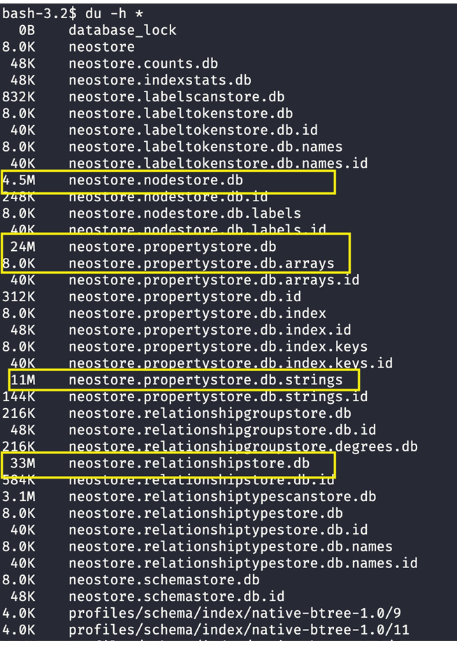
Figure 12.1 – Database store files
We can see from the screenshot that the store files are highlighted. These are the files that will have the most impact on the memory and performance requirements. We are discussing these aspects here because understanding how Neo4j stores and retrieves data helps us to write more optimal queries. The reason we are discussing this aspect in this chapter instead of earlier ones is that combining this knowledge and query processing with tips can better assist you to build queries. For example, if you have been working with Cypher queries and want to look at how to improve your skills, this chapter is more beneficial.
Let’s now look at node store structure.
Understanding the node store
A node store is a single file that stores all the nodes in a graph. Each node is a fixed-size data structure, as shown in the following table.
|
ID |
Labels |
Props |
Rels |
|
01 |
:Patient |
01 |
01 |
Table 12.2 – Node data structure
From the preceding table, we can see that the node data structure contains the node ID. This is an index in the node store file (nodestore.db) that we looked at in the previous section. It has labels associated with it. We can see in the table that this node has a label, Patient. The Props section contains the first property of the node. If there are other properties, they are stored as a linked list, with the first property being stored in the node. The Rels section points to the first relationship this node has. If the number of relationships starts becoming dense, such as more than 100, then this can point toward a relationship group store. The relationships also get connected as a linked list. When it is stored as a group, it will have one entry per relationship type, with IN and OUT directions separated. The labels stored are not the actual strings but, instead, ID numbers associated with the label name, and the corresponding ID is stored in the node data structure.
Now, let’s look at the relationship store.
Understanding the relationship store
The relationship data structure is a bit bigger than a node. It can be seen as follows:
|
ID |
Type |
Source node |
Target node |
Props |
Source previous |
Source next |
Target previous |
Target next |
|
01 |
HAS_ENCOUNTER |
01 |
03 |
09 |
6 |
02 |
4 |
03 |
Table 12.3 – Relationship data structure
The ID value is the index in the relationship store file (relationshipstore.db) that we looked at in the previous section. It has one type, which is an ID number associated with that name. It contains both Source node and Target node IDs in the data structure. This should make it clear that in Neo4j, data is connected as a doubly linked list to make it easier to traverse in any direction in an efficient manner. The properties section contains the ID of the first property associated with this relationship. The Source previous entry contains the number of relationships in the chain for the source node when this is the first relationship in the chain. Similarly, Target previous contains the number of relationships in the chain for the target node if this is the first relationship in the chain. This is useful to tell us the number of relationships the node is connected quickly with. If it is not the first relationship in the chain, then these entries will contain the previous relationship in the chain.
The Source next entry contains the next relationship for the source node in the chain. The same applies to the Target next entries. This should make it clear that once we have obtained the relationship, we can traverse back and forth using the previous and next entries, depending on the source or target node context.
Next, let us take a look at the property store.
Understanding the property store
The property store contains the property values for both nodes and relationships in a single stored file. It is split into three different stores to make sure the data structure size can be fixed.
Let us look at the basic property data structure:
|
ID |
NextProp |
PrevProp |
Payload |
|
01 |
02 |
-1 |
name | String | “Jon” |
Table 12.4 – Property data structure
Similar to node and relationship stores, ID is the index in the property store file (propertystore.db). It contains the locations to store next and previous properties. The Payload section contains the ID for the property name, the ID for the type, and the actual value. This can store all the basic property types except lists, which are stored in a property arrays store (propertystore.db.arrays).
One exception is that, if the string value does not fit into the data structure here, it will be stored in the string’s property store (propertystore.db.strings). In that case, the last value we stored in the payload points to the ID of the data structure stored in the strings property store or arrays property store. Even the strings property store and arrays property store use fixed-size data structures. If a value does not fit in one data structure, it can be split into a chain of data structures to store all the values. So, when you are storing a large string or reading it, the cost of it can be higher.
Note
As you can see from the previous paragraph, storing and retrieving large strings or arrays can be costly, as we may need to traverse multiple chain blocks to retrieve data. Therefore, we need to be careful about how and what we are storing and how we are retrieving the data.
You can read about data structure sizes here: https://neo4j.com/developer/kb/understanding-data-on-disk/.
Next, we will take a look at how Neo4j uses memory to execute queries.
Understanding Neo4j memory usage
Neo4j splits the memory into three different segments, given as follows:
- JVM memory: This is the memory used to load the Java classes, compiled Cypher queries, thread stacks, metaspace, GC, Lucene indices, and so on.
- Heap: This is the memory that is used to execute the queries. This contains the transaction state, query execution data, and graph management details. For high transactional usage, this should not exceed 31 GB because the JVM garbage collection is not efficient if the heap is more than that.
- Page cache: Cached graph data and indices.
When a query is executed, a transaction state is initiated in heap memory, and it goes to the page cache to retrieve the data. The query execution always goes to the page cache to get the nodes, relationships, and properties. If a node, relationship, or property is not found in the page cache, it causes a page fault that will load the required entity from the corresponding store. Since the page cache loads not just one data structure but a single page block around 4 KB, it may be reading more data than required.
You can read more about these aspects at https://www.graphable.ai/blog/neo4j-performance/ and https://maxdemarzi.com/2012/08/13/neo4j-internals/.
Now that we have taken a brief look at how Neo4j stores data, let’s look at some query patterns and review what a good query and a bad query are.
Reviewing querying patterns
Let’s review a few query patterns and see how a database will try to execute them to understand how to write optimal queries:
- The following code segment shows one of the most common mistakes:
MATCH (Mango {color: 'Yellow'}) return count(*)
We forgot to add :, even if Mango is a valid label. When we look at the query, we read it as return the count of yellow mangoes. Say we have mangoes, oranges, and apples in our cart. Since a database does not know what a mango is, it is going through all the fruits and checking for a color property, which should be Yellow, and returns the count of that. This is because when the database sees the query, it does not see the name Mango as a label.
Tip
Look for browser warnings before running the queries. Browsers are very good at highlighting these kinds of errors.
- The following code block is another common mistake made by developers:
MATCH (p:Patient)--(e:Encounter) RETURN p,e
There are two issues here. First, no direction is provided for the relationship. Second, there is no relationship type provided. Let’s see whether we can explain, in layman’s terms, the work the database needs to do here. Let’s say there is a junction with four incoming roads and three outgoing roads. There is a post office one block away. If someone asks us to find the post office one block away, since we don’t know where it is, we have to traverse all the roads by one block to find the post office. That’s what the database is doing here. It is traversing one hop in all directions and giving you data. Let’s see how this changes if a direction was provided. If we are looking for the post office one block away on the outgoing roads, we would be looking at only three roads instead of seven roads. This is the same with the database. Let’s see how this changes if there was more information provided. Out of the three roads, let’s say two are going east and one is going west. If we are asked to find a post office one block away on eastward outgoing roads, then we will be looking at only two roads instead of three. Similarly, if we provide the relationship type, then the amount of work the database does to retrieve data is also less.
Tip
Look at the query profile to understand the amount of work the database is doing. We should always be using the direction and relationship type for better performant queries.
- The following query can be very expensive in terms of memory and CPU usage. Depending on the graph size, this can cause out-of-memory exceptions and can crash a database server:
MATCH path=(:Patient)-[*]-(:Drug) RETURN path
Again, if we use the layman example from before, this is like trying to find a post office from a given point. This means we have to traverse in all directions and find all the paths that connect this point and a post office. Say you are at a point in a city and traversing all the roads in all directions to find all the paths; you can imagine how much time and effort it would take. Almost the same thing is happening here with the database. These kind of queries should be avoided at all costs. This query should have used relationship types, direction, and limiting the length to be able to respond in time.
Tip
You can avoid having out-of-memory exceptions thus causing outage by using the dbms.memory.transaction.global_max_size configuration. This configuration makes sure that all queries will not use more memory than this value. This should be a bit smaller than the maximum heap size configured. Also, you can use dbms.memory.transaction.max_size to make sure a given query does not use more than this memory. If it tries to use more memory, it would be terminated.
Cypher queries can be termed as anchor and traverse. Anchor means we are finding a node from which we start our traversal of a graph. This is the strongest feature of Neo4j.
In general, the following rules help to write better queries.
- For the anchoring point, make sure there is an index created for the WHERE condition. Remember that in Neo4j, a node label and property name are part of the index.
- We should traverse from a node that has a fewer number of relationships.
- It is always better to use direction and relationship types in queries; unless we want to traverse all the relationships, the node has to do our work.
- Leverage count stores for performant queries.
- Avoid specifying the labels for the nodes in the path, if possible, except the anchor node. This adds one extra step to do during traversal. In general, with a good model, the relationship type indicates what the next node label would be.
- Profile queries to understand the amount of work a database is doing.
- Leverage certain properties, such as true or false or values that contain a group with a limited set of values, to labels on the node. Using these labels can be much more effective than checking for a property or relying on an index.
- Property access is the most expensive part of Neo4j queries. Delay accessing the properties as late as you can.
- Make sure you are leveraging index-based sorting in your queries.
- Do not start the traversal from a super node. You can always check whether a node is connected to a super node.
- Use constraints, such as unique constraints, for nodes if possible. This can make a query optimizer pick an optimal query plan, instead of a simple index.
- Be careful when using variable length expansion. If possible, use bounds to limit the expansion. Also, for complex traversals, leverage apoc.path.expandConfig.
- Leverage apoc procedures and functions.
- Pay attention to how your graph is growing. The most common mistake made in data modeling is relying heavily on properties, which means we will also be relying on index lookups more often. This leads to a smaller graph in terms of node and relationship store sizes, and bigger property and index stores.
Next, we will take a look at troubleshooting a few common issues.
Troubleshooting a few common issues
When you are troubleshooting, logs are your friends. You must take a look at query log and debug log files to identify any issues. Please note that query logs are not available in Community Edition of Neo4j. If you are using Neo4j Desktop to create a database and test it, then you are using a single-user enterprise license, so you will have access to query logs. We will take a look at what information we have to troubleshoot issues and how we can fix them here:
- A debug log tells you a lot about how memory is being used. Look out for JVM garbage collection (GC) pauses. If there are few GC pauses and they are smaller than 100 ms, then there should not be any issues. If there are lot of GC pauses and they are going above 100 ms, then the queries are using lot of heap. This could be due to a bad query, no indexes, or a query collecting a lot of data.
- Query logs tell you how much time a query is taking. If you enable time tracking using dbms.logs.query.time_logging_enabled, you can see the actual CPU time the query has taken, along with the amount of time it spent waiting for resources to become available and the time taken to create a plan. By enabling dbms.logs.query.page_logging_enabled, you can also see the number of page faults the query is causing:
- If a lot of queries have a plan time greater than 0, then you might not be leveraging parameterization of queries.
- If a query has more than zero wait time, then you may not have enough compute power to handle the queries. This, by itself, should not be an issue if the wait time is small – say, under 100 ms. When you get a burst of queries at the same time, some of the queries do have to wait for the CPU to be available. It is also possible that the query is waiting for another transaction to complete because it is trying to modify the same node or relationship and needs to acquire a lock on it. Again, if the wait time is small, then it should not be an issue.
- If a lot of queries have page faults, then the page cache available may not be enough. We need to understand how our queries are using the page cache to make sure we reduce the page faults. Most likely, the situation here would be that your data model has evolved and your queries may not be efficient any more. Another situation could be your queries are over-reliant on properties, and the page cache is not big enough to hold a property store along with node and relationship stores.
Let’s take a look at few of the common issues faced during query execution and how to address them:
- The write query performance starts degrading as we keep writing data: The most likely scenario here is that there are no indexes created. As the data keeps growing, the time taken to find a node for a given label linearly keeps increasing:
- Take a look at your MERGE and MATCH statements to make sure you are leveraging indexes using EXPLAIN
- An out-of-memory exception during writes: This means that the heap provided is not enough to handle the request:
- If you are using the LOAD CSV command, then use EXPLAIN to see whether there are any EAGER steps. If there are any EAGER steps, then the query engine tries to load all the CSV data into memory before it can start processing it. If you are trying to load a large file, then it can run out of memory.
The best way to resolve this issue is to change the query to avoid any EAGER steps. Please read this article about it: https://medium.com/neo4j/cypher-sleuthing-the-eager-operator-84a64d91a452. Another option is to use client drivers and avoid using LOAD CSV in production environments. This should be your approach for stable applications.
- Check whether the heap is good by reducing the batch size.
- An out-of-memory exception during read queries: This means the query is collecting a lot of data in memory before it can start returning it. This is the most common scenario if you are using COLLECT, ORDER BY, or DISTINCT clauses:
- A MERGE query creating duplicate nodes: MERGE is supposed to check whether the node exists and creates it only if it does not exist. However, this operation is not thread-safe. If you have two separate transactions that are executing this statement at the same time, then it is possible to have duplicate nodes:
- If it is possible, create a unique constraint on the key used in the MERGE statements. It may cause one of the transactions to fail, but there won’t be any duplicates.
- A MERGE statement is failing with a unique constraint error: A MERGE statement tries to create the whole path, excluding variables. Let’s say your query is as follows:
MERGE (p:Person {id:1})-[:LIVES_AT]->(:Address {id:"A1"})
Here, even if the Person and Address nodes exist, if there is not a relationship between them, then MERGE will try to create the whole path, which means creating the Person and Address nodes again.
- The best way to address this is to split the query into the following:
MERGE (p:Person {id:1})MERGE (a:Address {id:"A1"})MEGE (p)-[:LIVES_AT]->(a)
This query is doing MERGE on the nodes first and separates the relationship creation using another MERGE statement. Since they are separated, this query will not attempt to create duplicate nodes.
- An application shows the Unable to schedule bolt session <session_id> for execution since there are no available threads to serve it at the moment error. This means the server bolt connection thread pool is exceeded. This can be due to bad coding, where the sessions are not closed, there is burst traffic that is exceeding the thread pool configuration, or queries are taking time and the connections are not being released in time:
- Check the client code to make sure that after the transaction is complete, session.close() is called
- If the traffic rate is higher than the connection pool available, then increase the bolt thread pool size on the server
- Check whether the queries are performing well and that they are not blocking the resources for a long time
- In the cluster, all the queries are going to the leader node. This means the client code is using the session.run() method to execute the queries. This implicitly creates a write transaction and all those transactions go to the leader. Also, the applications built using the Spring Data framework, by default, start to write transactions. In this case, again, all your queries are directed to the leader node:
- If you are using a driver directly in the client, then you should use the session.readTranasaction() and session.writeTransaction() methods. In this case, all the read queries are directed to follower nodes and writes are directed to leader node.
- If you are using the Spring Data framework, annotate the methods that should be executing read queries using the @Transaction(readonly=true) annotation.
- Queries are slow in Enterprise Edition. In some scenarios, queries work fine in Community Edition of Neo4j but are slow in Enterprise Edition:
- Neo4j Community Edition supports only interpreted runtimes. In this mode, a basic plan is used to execute queries. In Enterprise mode, there are optimized runtimes such as pipelined and slotted. In Enterprise mode, by default, the query planner tries to use pipelined mode, which tries to optimize for faster execution. It is possible in a few scenarios that the query planner makes a mistake and the pipelined runtime is not effective. In these scenarios, it is possible to tell the planner to use other runtimes. One of the ways to force runtime is to prefix the query with CYPHER runtime=interpreted. When the planner sees this, it tries to use the runtime that is requested.
Note
This option is only available in Enterprise mode. Also, from 5.0 onward, the slotted runtime is the default option in Community Edition, and interpreted runtime is not available. You can read more about these options at https://neo4j.com/docs/cypher-manual/4.4/query-tuning/how-do-i-profile-a-query/.
- Queries are slow and there are lot of page faults: This means that the page cache is not enough to be able to execute the queries efficiently. Most likely, the situation here is that the graph data model evolved too quickly or is not in an optimal state. Another situation is that we are over-reliant on properties and indexes, and that is requiring a lot of page cache:
- Take a look at your store sizes and your query patterns to see whether the page cache settings are optimal.
- If the node store and relationship store are very small and the property and index stores are bigger, then we are over-reliant on properties and indexes. We need to take a step back and see whether the model can be improved. Another aspect to look at here is whether we can make the queries easy to traverse and access properties at the end.
Next, let’s take a look what’s new in Cypher 5.0.
Reviewing the new 5.0 changes
In version 5.0, multiple changes have been made to the Cypher language. You can read about all these changes at https://neo4j.com/docs/cypher-manual/current/deprecations-additions-removals-compatibility/. We will take a look few of the changes that impact the Cypher queries.
The first important change to note is index creation. In version 5.0, the indexes are separated to represent the different types so that the indexes can be more performant. The indexing types that are available in version 5.0 are listed here:
- Fulltext index: This is the Lucene text index
- Lookup index: This index is for node labels and relationship types
- Range index: This index replaces the B-tree index option and can be used with a single or multiple properties
- Text index: This index is used on string properties
- Point index: This index is used on point types
You can read more about the new index types at https://neo4j.com/docs/cypher-manual/current/indexes-for-search-performance/.
Another change that could be important for developers applies to label filtering and relation type filtering, along with the WHERE clause. It is possible to use logical predicates for node label and relationship types.
Here’s a sample query that demonstrates this aspect:
MATCH (n: A&(B|C)&!D|E) RETURN n
You can see in this query that we want all the nodes with E or A labels, either B or C, and not D.
It is also possible to use the same syntax for relationships.
Here’s a sample query that demonstrates this aspect:
MATCH p=()-[: A&(B|C)&!D|E]->() RETURN p
The logic here is also very similar to how node label filtering works.
Another change that is interesting is that we can use the WHERE clause in line with node labels and relationship types.
Here’s an example of inline usage with nodes:
MATCH (a:Person WHERE a.name = 'Rob')
      -[:KNOWS]->(b:Person WHERE b.age > 25)
RETURN b.name
We can see the WHERE clause is used in line with nodes.
The same syntax also applies to relationships:
MATCH (a:Person {name: 'Tom'})
RETURN [(a)
-[r:KNOWS WHERE r.since < 2020]->(b:Person) | r.since] AS years
We can see that we are able to use the WHERE clause in line with the relationship that is inside a list comprehension. This new syntax can help us build complex queries with ease.
You can read more about this syntax and examples at https://neo4j.com/docs/cypher-manual/current/clauses/where/.
One last thing that may impact how users can add configuration to the neo4j.conf file is the introduction of a new configuration parameter called server.config.strict_validation.enabled. This is, by default, set to true. What this configuration does is not start the database instance if there are unknown configuration namespaces that are not part of the core database configuration, such as apoc, or a configuration is repeated multiple times, and then the database will fail to start. This is more of a security feature. So, when you want to add a new configuration, such as apoc.import.file.enabled=true, it would cause a problem.
There are two options available when you run into this kind of scenario:
- Modify the configuration to add or update the value to server.config.strict_validation.enabled false, as shown here:
server.config.strict_validation.enabled=false
- Create a separate configuration file that is appropriate for the plugin you are loading and add the configuration there. For example, for the apoc plugin, you can add all apoc-related configurations to the apoc.conf file and add it to the configuration directory.
A sample apoc.conf configuration would look like this:
apoc.import.file.enabled=true apoc.import.file.use_neo4j_config=false
Please note that in the new configuration file, you need to add the apoc.import.file.use_neo4j_config=false config for the apoc plugin to use this new configuration file. If not, it looks for the configuration in the neo4j.conf file.
Now, let’s summarize everything we have learned.
Summary
In this chapter, we took a deeper look at Neo4j internals to understand how a database works to execute queries. We also reviewed a few query patterns and saw the right and wrong ways to build queries and looked at troubleshooting common issues.
Cypher is an easy language to learn compared to SQL. However, it takes a bit of an effort to get the most out of it. One thing to remember is that Neo4j is a schemaless storage. This gives us great flexibility when it comes to data modeling. If your application use case starts changing, the current data model becomes too limiting, and your queries get slower, there is no need to create a completely new model. You can start adapting the existing model by adding new model concepts, thus keeping the same graph for the old and new functionality. Once you are satisfied with new model changes, it is possible to remove the remnants of the old model that are not required. Combining this kind of model flexibility with the simplicity and power of Cypher makes it easy to build effective and complex applications.
Furthermore, openCypher, which is the open source version of the Cypher language, is being adapted by other graph databases such as Amazon Neptune. So, by learning Cypher, your knowledge is not just limited to Neo4j but can also be leveraged to work with other databases. However, there might be subtle nuances that you need to be aware of to get the most out of different types of graph databases.
In short, to become an effective Cypher query developer, understand the domain and take a look at the graph database capabilities and graph modeling. Also, become familiar with capabilities such as EXPLAIN and PROFILE along with logs that are available to be able to identify and fix any issues.