So, let's move along!

We will now take a look at plotting some of the data we collected in our Spark DataFrame. You can use matplotlib and pandas to create almost an endless number of visualizations (once you understand your data well enough).

You may even find that, once you reach this point, generating visualizations is quite easy but then you can spend an almost endless amount of time getting them clean and ready to share with others.

We will now look at a simple example of how this process might go.

Starting with the Spark DataFrame from the previous section, suppose that we think that it would be nice to generate a simple bar chart based upon the DATE field within our data. So, to get going, we can use the following code to come up with a count by DATE:

df_data_2.groupBy("DATE").count().show()
df_data_2.groupBy("DATE").count().collect()

The results of running the preceding code are shown in the following screenshot:

We might say that the output generated seems somewhat reasonable (at least at first glance), so the next step would be to use the following code to construct a matrix of data formatted in a way that can easily be plotted:

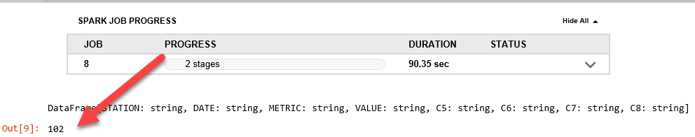
count = [item[1] for item in df_data_2.groupBy("DATE").count().collect()]
year = [item[0] for item in df_data_2.groupBy("DATE").count().collect()]
number_of_metrics_per_year = {"count":count, "DATE" : year}
import pandas as pd
import matplotlib.pyplot as plt
%matplotlib inline
number_of_metrics_per_year = pd.DataFrame(number_of_metrics_per_year )
number_of_metrics_per_year .head()

Running this code and looking at the output generated seems perfectly reasonable and in line with our goal:

So, great! If we got to this point, we would think that we are ready to plot and visualize the data, so we can go ahead and use the following code to create a visualization:

number_of_metrics_per_year = number_of_metrics_per_year.sort_values(by = "DATE")
number_of_metrics_per_year.plot(figsize = (20,10), kind = "bar", color = "red", x = "DATE", y = "count", legend = False)
plt.xlabel("", fontsize = 18)
plt.ylabel("Number of Metrics", fontsize = 18)
plt.title("Number of Metrics Per Date", fontsize = 28)
plt.xticks(size = 18)
plt.yticks(size = 18)
plt.show()

After running the preceding code, we can see that the code worked (we have generated a visualization based upon our data) yet the output isn't quite as useful as we might have hoped:

It's pretty messy and not very useful!

So, let's go back and try to reduce the volume of data we are trying to plot. Thankfully, we can reuse some of the code from the previous sections of this chapter.

We can start by again setting up a temporary table that we can query:

from pyspark.sql import SQLContext
sqlContext = SQLContext(sc)
df_data_2.registerTempTable("MyWeather")

Then, we can create a temporary DataFrame to hold our results (temp_df). The query can only load records where METRIC collected is PRCP and VALUE is greater than 500:

temp_df =  sqlContext.sql("select * from MyWeather where METRIC = 'PRCP' and VALUE>500")
print (temp_df)
temp_df.count()

This should significantly limit the number of data records to be plotted.

Now we can go back and rerun our codes that we used to create the data matrix to be plotted as well as the actual plotting code but, this time, using the temporary DataFrame:

temp_df.groupBy("DATE").count().show()
temp_df.groupBy("DATE").count().collect()
count = [item[1] for item in temp_df.groupBy("DATE").count().collect()]
year = [item[0] for item in temp_df.groupBy("DATE").count().collect()]
number_of_metrics_per_year = {"count":count, "DATE" : year}
import pandas as pd
import matplotlib.pyplot as plt
%matplotlib inline
number_of_metrics_per_year = pd.DataFrame(number_of_metrics_per_year )
number_of_metrics_per_year .head()
number_of_metrics_per_year = number_of_metrics_per_year.sort_values(by = "DATE")
number_of_metrics_per_year.plot(figsize = (20,10), kind = "bar", color = "red", x = "DATE", y = "count", legend = False)
plt.xlabel("", fontsize = 18)
plt.ylabel("Number of Metrics", fontsize = 18)
plt.title("Number of Metrics Per Date", fontsize = 28)
plt.xticks(size = 18)
plt.yticks(size = 18)
plt.show()

So now we have a different, maybe somewhat better, result but one that is probably still not ready to be shared:

If we continue using the preceding strategy, we could again modify the SQL query to further restrict or filter the data as follows:

temp_df =  sqlContext.sql("select * from MyWeather where METRIC = 'PRCP' and VALUE > 2999")
print (temp_df)
temp_df.count()

And then we can review the resulting temporary DataFrame and see that now it has a lot fewer records:

If we now proceed with rerunning the rest of the plotting code, we see that it yields a slightly better (but still not acceptable) plot:

We could, in fact, continue this process of trial and error by modifying the SQL, rerunning the code, and then reviewing the latest results until we are happy with what we see, but you should have the general idea, so we will move on at this point.