4	Human Information Processing

Information processing lies at the heart of human performance. In a plethora of situations in which humans interact with systems, the operator must perceive information, transform that information into different forms, take actions on the basis of the perceived and transformed information, and process the feedback from that action, assessing its effect on the environment.

C. D. Wickens & C. M. Carswell
2012

INTRODUCTION

The human information-processing approach to studying behavior characterizes the human as a communication system that receives input from the environment, acts on that input, and then outputs a response back to the environment. We use the information-processing approach to develop models that describe the flow of information in the human, in much the same way that system engineers use models to describe information flow in mechanical systems. The similarity between the human information-processing and system perspectives is not coincidental; the human information-processing approach arose from the contact that psychologists had with industrial and communication engineers during World War II.

Information-processing concepts have been influenced by information theory, control theory, and computer science (Posner, 1986). However, experimental studies of human performance provide the empirical base for the approach. An information processing account of performance describes how inputs to the perceptual system are coded for use in cognition, how these codes are used in different cognitive subsystems, the organization of these subsystems, and mechanisms by which responses are made. Diagrams of hypothesized processing subsystems can identify the mental operations that take place in the processing of various types of information as well as the specific control strategies adopted to perform the tasks.

Figure 4.1 shows a simple example of an information-processing model. This model explains human performance in a variety of tasks in which responses are made to visually presented stimuli (Townsend & Roos, 1973). The model consists of a set of distinct subsystems that intervene between the presentation of an array of visual symbols and the execution of a physical response to the array. The model includes perceptual subsystems (the visual form system), cognitive subsystems (the long-term memory components, the limited-capacity translator, and the acoustic form system), and action subsystems (the response-selection and response-execution systems). The flow of information through the system is depicted by the arrows. In this example, information is passed between stages and subsystems.

FIGURE 4.1A model for performance of visual information processing.

Engineers can look inside a machine to figure out how it works. However, the human factors expert cannot look inside a person’s head to examine the various subsystems that underlie performance. Instead, he must infer how cognitive processing occurs on the basis of behavioral and physiological data. There are many models that he can consider, which differ in the number and arrangement of processing subsystems. The subsystems can be arranged serially, so that information flows through them one at a time, or in parallel, so that they can operate simultaneously. Complex models can be hybrids that are composed of both serial and parallel subsystems. In addition to the arrangement and nature of the proposed subsystems, the models also must address the processing cost (time and effort) associated with each subsystem.

Using these kinds of models, we can make predictions about how good human performance will be under different stimuli and environmental conditions. We evaluate the usefulness of any model by comparing its predictions with experimental data. The models that are most consistent with the data are more credible than alternative models. However, credible models must do more than simply explain a limited set of behavioral data. They must also be consistent with other behavioral phenomena and with what we know about human neurophysiology. In keeping with the scientific method, we will revise and replace models as we gather additional data.

The importance of the information-processing approach for human factors is that it describes both the operator and the machine in similar terms (Posner, 1986). A common vocabulary makes it easier to treat the operator and the machine as an integrated human–machine system. For example, consider the problem of a decision-support system in an industrial control setting (Rasmussen, 1986). The system assists operators during supervisory tasks and emergency management by providing information about the most appropriate courses of action in a given circumstance. Whether or not system performance is optimal will depend on the way the system presents information about the machine and the way the operator is asked to respond. The more useful and consistent this information is, the better the operator will be able to perform. Models of human information processing are prerequisites for the conceptual design of such systems, because these models can help determine what information is important and how best to present it (McBride & Schmorrow, 2005; Rasmussen, 1986). In human–computer interaction in particular, information-processing models have resulted in solutions for a range of issues (Proctor & Vu, 2012). Card, Moran, and Newell (1983, p. 13) note, “It is natural for an applied psychology of human-computer interaction to be based theoretically on information-processing psychology.”

Because “human society has become an information processing society” (Sträter, 2005), the information-processing approach provides a convenient framework for understanding and organizing a wide variety of human performance problems. It gives a basis for analyzing the components of a task in terms of their demands on perceptual, cognitive, and action processes. In this chapter, we will introduce the basic concepts and tools of analysis that are used in the study of human performance.

A THREE-STAGE MODEL

Figure 4.2 presents a general model of information processing that distinguishes three stages intervening between the presentation of a stimulus and the execution of a subsequent response. Early processes associated with perception and stimulus identification are in the perceptual stage. Following this stage are intermediate processes involved with decision making and thought: the cognitive stage. Information from this cognitive stage is used in the final action stage to select, prepare, and control the movements necessary to effect a response.

FIGURE 4.2Three stages of human information processing.

The three-stage model provides an effective organizational tool, which we will use in this book. Keep in mind that the model fails to capture preparatory processes that occur prior to the presentation of a stimulus (i.e., how a person anticipates or gets set to perform a particular task), as well as the intimate and cyclical relation between action and perception (e.g., Knoblich, 2006). Researchers who study human performance are interested in determining to which processing stage experimental findings should be attributed, and in characterizing information flow within the system. However, the boundaries between perception, cognition, and action are not as clearly defined as is implied by the model. It is not always clear whether a change in performance should be attributed to the perceptual, cognitive, or action stage. Once a specific change in performance can be clearly attributed to a stage, detailed models of the processing within that stage can be developed.

PERCEPTUAL STAGE

The perceptual stage includes processes that operate from the stimulation of the sensory organs (e.g., Wolfe et al., 2015). Some of this processing might occur without the person even becoming aware of it through the processes involved in the detection, discrimination, and identification of the stimulation. For example, a visual display produces or reflects patterns of light energy that are absorbed by photoreceptors in the eye (see Chapter 5). This triggers a neural signal that travels to areas of the brain devoted to filtering the signal and extracting information contained in it, such as shape, color, or movement. The ability of the brain to extract information from the signal depends on the quality of the sensory input. This quality is determined by, among other things, the clarity and duration of the display.

If the display is not clear, much of the information will be lost. When a film projector is poorly focused, you cannot see the details of the picture. Similarly, a poorly tuned television picture can be snowy and blurred. Displays that are presented very briefly or that must be examined very quickly, such as road signs and some computer error messages, do not allow the extraction of much information during the time that they are available. Such degradations of input to the sensory system restrict the amount of information that can be extracted and, thus, will restrict performance.

COGNITIVE STAGE

After the perceptual stage has extracted enough information from a display to allow the stimulus to be identified or classified, processes begin to operate with the goal of determining the appropriate action or response. These processes might include the retrieval of information from memory, comparisons among displayed items, comparison between these items and the information in memory, arithmetic operations, and decision making (e.g., Groome & Eyesenk, 2016). The cognitive stage imposes its own constraints on performance. For example, people are not generally very good at paying attention to more than one source of information or performing complicated calculations in their heads.

Errors in performance may arise from these and a number of other cognitive limitations. We often characterize cognitive limitations in terms of cognitive resources: If there are few available resources to devote to a task, then task performance may suffer. One of our goals as human factors specialists is to identify the cognitive resources necessary for the performance of a task and systematically remove limitations associated with these resources. This may require additional information displays, redesigning machine interfaces, or even redesigning the task itself.

ACTION STAGE

Following the perceptual and cognitive stages of processing, an overt response (if required) is selected, programmed, and executed (e.g., Schneider, 2015). Response selection is the problem of choosing which of several alternative responses is most appropriate under the circumstances. After a response is selected, it then must be translated into a set of neuromuscular commands. These commands control the specific limbs or effectors that are involved in making the response, including their direction, velocity, and relative timing.

Selection of the appropriate response and specification of the parameters of the movement take time. We usually see that the time required to begin a movement increases as the difficulty of response selection and movement complexity increase (Henry & Rogers, 1960). The action stage therefore imposes its own limitations on performance, just as the cognitive stage imposes limitations. There are also physical limitations that must be considered: An operator cannot press an emergency button at the same time as she is using both hands to close a valve, for example. Action stage limitations can result in errors in performance, such as the failure of a movement to terminate accurately at its intended destination.

HUMAN INFORMATION PROCESSING AND THE THREE-STAGE MODEL

The three-stage model is a general framework that we are using to organize much of what we know about human capabilities. It enables us to examine performance in terms of the characteristics and limitations of the three stages. This simple classification of human information processing allows a more detailed examination of the processing subsystems within each stage. For example, Figure 4.3 shows how each of the stages can be further partitioned into subsystems whose properties can then be analyzed. Box 4.1 describes more general cognitive architectures and the computational models we can develop from them based on detailed specifications of the human information-processing system.

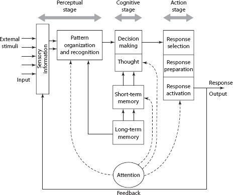
FIGURE 4.3An elaborated model of human information processing.

There are three kinds of processing limitations that can cause processing errors at each stage: data, resource, and structural limitations (Norman & Bobrow, 1975). Data-limited processing takes place when the information input to a stage is degraded or imperfect, such as when a visual stimulus is only briefly flashed or when speech signals are presented in a noisy environment. Resource-limited processing occurs if the system is not powerful enough to perform the operations required for a task efficiently, such as the memory resources required to remember a long-distance phone number until it is dialed. Structurally limited processing arises from an inability of one system to perform several operations at once. Structural limitations can appear at any stage of processing, but the most obvious effects occur in the action stage when two competing movements must be performed simultaneously with a single limb.

Although Norman and Bobrow’s distinction between different kinds of processing limitations may not accurately characterize the ways that cognitive processing can be realized in the human brain, it is a useful taxonomy. With this taxonomy, it becomes easier to determine whether performance limitations are due to problems in the way that information is being delivered to the operator, the kinds of information being used for a task, or components of the task itself. Furthermore, although it is easiest to see data limitations in the perceptual stage, resource limitations in the cognitive stage, and structural limitations in the action stage, it is important to remember that all three of these limitations may appear at any stage of processing.

PSYCHOLOGICAL REPRESENTATION OF THE PHYSICAL WORLD

Viewing the human being as an information-processing system is not a new idea in human factors and psychology. We can trace similar ideas as far back as the work of Ernst Weber and Gustav Fechner in the 1800s, discussed in Chapter 1, and even farther. The information-processing view brings with it a number of questions, two of which we address in this section. These are (1) what are the limits of the senses to sensory stimulation, and (2) how do changes in stimulus intensity relate to changes in sensory experience? Researchers who concern themselves with answering these kinds of questions are called psychophysicists. Many psychophysical techniques have been developed to measure sensory experience (e.g., Kingdom & Prins, 2010; Szalma & Hancock, 2015), and these techniques are a valuable part of every competent human factors specialist’s toolbox.

Most psychophysical techniques rely on the frequency with which certain responses are made under different stimulus conditions. For example, we might be concerned with the number of times a radiologist sees a shadow on the X-ray of someone’s lung under different lighting conditions. The frequency of times a shadow is reported can be used to infer properties of the sensory experience provided by a particular X-ray, lighting scheme, and so on.

The psychophysical methods that we discuss here provide precise answers to questions about detectability, discriminability, and perceived magnitude for almost any conceivable kind of stimulus. Detectability refers to the absolute limits of the sensory systems to provide information that a stimulus is present. Discriminability involves the ability to determine that two stimuli differ from each other. Discovering the relation between perceived magnitude and physical magnitude is referred to as psychophysical scaling.

Most of what we know about the dynamic ranges of the human senses and the precise sensory effects of various physical variables, such as the frequency of an auditory stimulus, was discovered using psychophysical techniques. These techniques also have been used to investigate applied issues in many areas, although perhaps not as widely as is warranted. The importance of using psychophysical methods to study applied problems was stressed by Uttal and Gibb (2001), who conducted psychophysical investigations of night-vision goggles. They concluded that their work supports the general thesis that “classical psychophysics provides an important means of understanding complex visual behavior, one that is often overlooked by both engineers and users” (p. 134). It is important to realize that basic psychophysical techniques can be used by human factors specialists to solve specific problems relating to optimal design.

CLASSICAL METHODS FOR DETECTION AND DISCRIMINATION

The most important concept in classical psychophysics is that of the threshold. An absolute threshold is the smallest amount of intensity a person needs to detect a stimulus (VandenBos, 2015). A difference threshold is the smallest amount of difference a person needs to perceive two stimuli as different. The goal of the classical psychophysical methods is to measure these thresholds accurately.

The definition of a threshold suggests fixed values below which stimuli cannot be detected or differences discriminated, and above which stimuli are always perfectly detected. That is, the relation between physical intensity and detectability should be a step function (illustrated by the dashed line in Figure 4.4). However, psychophysical studies always show a range of stimulus values over which an observer will detect a stimulus or discriminate between two stimuli only some percentage of the time. Thus, the typical psychophysical function is an S-shaped curve (as shown by the points in Figure 4.4).

FIGURE 4.4Proportion of detection responses as a function of stimulus intensity for idealized (dashed) and actual (points) observers.

Fechner developed the classical methods we use for measuring thresholds. Although many modifications to his procedures have been made over the years, the methods in this tradition still follow closely the steps that he outlined. These methods require us to make many measurements in carefully defined conditions, and we estimate the threshold from the resulting distribution of responses. Two of the most important methods are the method of limits and the method of constant stimuli (Kingdom & Prins, 2010).

To find an absolute threshold using the method of limits, we present stimulus intensities that bracket the threshold in a succession of small increments to an observer. For instance, to determine an observer’s threshold for detecting light, we could work with a lamp that can be adjusted from almost-zero intensity to the intensity of a 30-watt light bulb. We could start with an ascending sequence of intensities, beginning with the lowest intensity (almost zero) and gradually increasing the intensity. At each intensity level, we ask the observer whether he sees the light. We keep increasing the intensity until the observer reports that he has seen the light. We then compute the average of the intensities for that trial and the immediately preceding trial and call that the threshold intensity for the series. It is important to also present a descending series of trials, where we start with the highest intensity and decrease the intensity on each step. We must repeat this procedure several times, with half of the series being ascending and the other half being descending. For each series, we will obtain a value for the threshold. The average of all of the thresholds that we compute for a particular observer is defined as the absolute threshold for that observer.

To find difference thresholds with the method of limits, we present two stimuli on each trial. The goal is to determine the smallest difference between the two stimuli that the observer can detect. If we are still concerned with light intensities, we would need two lamps. The intensity of one lamp remains constant, and we call that intensity the standard. The intensity of the other lamp varies, and we call that intensity the comparison. On each trial, the observer must say whether the comparison stimulus is less than, greater than, or equal to the standard stimulus. We increment and decrement the intensity of the comparison in exactly the same way as we just described for determining the absolute threshold, and measure the intensities at which the observer’s response changes from less than to equal or from greater than to equal. These intensities define two thresholds, one for ascending and one for descending sequences. We could average the two thresholds to get an overall difference threshold, but it is common to find that the two thresholds obtained in this way are actually quite different, so averaging might not provide an accurate threshold value.

The second method is the method of constant stimuli. In contrast to the ascending and descending series of intensities presented in the method of limits, we present different intensities in random order. If we are still working with light intensities, the observer would report whether the light was seen on each trial, just as before. For each intensity, we compute the number of times that the light was detected, and the threshold intensity is defined as that intensity for which the light was detected 50% of the time. Figure 4.4 shows how the data might look for this procedure.

It is also easy to determine difference thresholds using the method of constant stimuli. Using two lamps, we again hold the intensity of the standard constant, but the intensity of the comparison varies randomly from trial to trial. The difference threshold is defined as the comparison intensity for which the observer reports 50% “greater than” and 50% “less than” responses.

The methods of limits and constant stimuli, as well as many others, have been used successfully since Fechner’s work to obtain basic, empirical information about the characteristics of each of the senses. It is important to understand that the measurement of a threshold in an isolated condition is not very informative. Rather, it is the changes in the threshold under varying conditions that provide critical information about sensory limitations. For example, the light intensity threshold we just described will depend on the color of the light (see Chapter 5). Also, the difference threshold that we compute will depend on the intensity of the standard: The higher the intensity of the standard, the higher the difference threshold will be. For auditory stimuli, the detection threshold is a function of the stimulus frequency; very high-pitched and very low-pitched sounds are more difficult to hear. Findings like these do not only reveal basic characteristics of the visual and auditory systems, but also provide information for the human factors specialist about how visual and auditory information should be presented to ensure that a person can perceive it.

In some situations, we might want to insure that people can’t perceive something. For example, Shang and Bishop (2000) evaluated the impact of introducing a transmission tower or oil refinery tanks into landscape settings. They edited photographs of landscapes to include these (ugly) structures and used psychophysical methods to obtain difference thresholds for detection, recognition, and visual impact (degradation of the views caused by the structure). They showed that the size of the structure and its contrast with the surroundings determined all three threshold types. The authors recommended extension of threshold measurement to assess the aesthetic effects of other types of changes to the environment, such as billboards and clearcuts.

Despite their utility, there are several problems with the threshold concept and the methods used to evaluate it. Most serious is the fact that the measured value for the threshold, which is assumed to reflect sensory sensitivity, may be affected by the observer’s desire to say yes or no. Some evidence for this is the common finding that the difference threshold is not the same for ascending and descending sequences. Consider the extreme case, where a person decides to respond yes on all trials. In these circumstances, no threshold can be computed, and we have no way of knowing whether she actually detected anything at all. We could address this problem by inserting some catch trials on which no stimulus is presented. If she responds yes on those trials, her data could be thrown out. However, catch trials will not pick up response biases that are less extreme.

SIGNAL-DETECTION METHODS AND THEORY

The problem with the classical methods is that threshold measurements are subjective. That is, we have to take the observer’s word that she detected the stimulus. This is like taking an exam that consists of the instructor asking you whether or not you know the material and giving you an A if you say “yes.” A more objective measure of how much you know requires that that your “yes” response be verified somehow. An objective test can be used that requires you to distinguish between true and false statements. In this case, the instructor can evaluate your knowledge of the material by the extent to which you correctly respond yes to true statements and no to false statements. Signal-detection methods are much like an objective test, in that the observer is required to discriminate trials on which the stimulus is present from trials on which it is not.

Methods

In the terminology of signal detection (Green & Swets, 1966; MacMillan & Creelman, 2005), noise trials refer to those on which a stimulus is not present, and signal-plus-noise trials (or signal trials) refer to those on which a stimulus is present. In a typical signal-detection experiment, we select a single stimulus intensity and use it for a series of trials. For example, the stimulus may be a tone of a particular frequency and intensity presented in a background of auditory noise. On some trials we present only the noise, whereas on other trials we present both the signal and the noise. The listener must respond yes or no depending on whether he heard the tone. The crucial distinction between the signal-detection methods and the classical methods is that the listener’s sensitivity to the stimulus can be calibrated by taking into account the responses made when the stimulus is not present.

Table 4.1 shows the four combinations made up of the two possible states of the world (signal, noise) and two responses (yes, no). A hit occurs when the observer responds yes on signal trials, a false alarm when the response is yes on noise trials, a miss when the response is no on signal trials, and a correct rejection when the response is no on noise trials. Because the proportions of misses and correct rejections can be determined from the proportions of hits and false alarms, signal-detection analyses typically focus only on the hit and false-alarm rates. You should note that this 2 × 2 classification of states of the world and responses is equivalent to the classification of true and false null hypotheses in inferential statistics (see Table 4.2); optimizing human performance in terms of hits and false alarms is the same as minimizing Type I and Type II errors, respectively. The key to understanding signal-detection theory is to realize that it is just a variant of the statistical model for hypothesis testing.

TABLE 4.1

Classifications of Signal and Response Combinations in a Signal-Detection Experiment

Response	State of the World
	Signal	Noise
“Yes” (present)	Hit	False alarm
“No” (absent)	Miss	Correct rejection

A person’s sensitivity to the stimulus is good if his hit rate is high and his false-alarm rate low. This means that he makes mostly yes responses when the signal is present and mostly no responses when it is not. Conversely, his sensitivity is poor if the hit and false-alarm rates are similar, so that he responded yes about as often as he responded no regardless of whether or not a signal was presented. We can define several quantitative measures of sensitivity from the hit and false-alarm rates, but they are all based on this general idea.

Sometimes a person might tend to make more responses of one type than the other regardless of whether the signal is present. We call this kind of behavior a response bias. If we present the same number of signal trials as noise trials, an unbiased observer should respond yes and no about equally often. If an observer responds yes on 75% of all the trials, this would indicate that he has a bias to respond yes. If no responses are more frequent, this would indicate that he has a bias to respond no. As with sensitivity, there are several ways that we could quantitatively measure response bias, but they are all based on this general idea.

Theory

Signal-detection theory provides a framework for interpreting the results from detection experiments. In contrast to the notion of a fixed threshold, signal-detection theory assumes that the sensory evidence for the signal can be represented on a continuum. Even when the noise alone is presented, some amount of evidence will be registered to suggest the presence of the signal. Moreover, this amount will vary from trial to trial, meaning that there will be more evidence at some times than at others to suggest the presence of the signal. For example, when detecting an auditory signal in noise, the amount of energy contained in the frequencies around that of the signal frequency will vary from trial to trial due to the statistical properties of the noise-generation process. Even when no physical noise is present, variability is introduced by the sensory registration process, neural transmission, and so on. Usually, we assume that the effects of noise can be characterized by a normal distribution.

Noise alone will tend to produce levels of sensory evidence that are on average lower than the levels of evidence produced when a signal is present. Figure 4.5 shows two normal distributions of evidence, the noise distribution having a smaller mean μ _N than the signal distribution, which has a mean of μ _S + N. In detection experiments, it is usually not easy to distinguish between signal and noise trials. This fact is captured by the overlap between the two distributions in Figure 4.5. Sometimes noise will look like signal, and sometimes signal will look like noise. The response an observer makes on any trial will depend on some criterion value of evidence that she selects. If the evidence for the presence of the signal exceeds this criterion value, then she will respond “yes,” the signal is present; otherwise, she will respond “no.”

FIGURE 4.5Signal and noise distributions of sensory evidence illustrating determination of dʹ.

Detectability and Bias

We have explained in general terms what we mean by sensitivity (or detectability) and response bias. Using the framework shown in Figure 4.5, we now have the tools needed to construct quantitative measurements of detectability and bias. In signal-detection theory, the detectability of the stimulus is reflected in the difference between the means of the signal and noise distributions. When the means are identical, the two distributions are perfectly superimposed, and there is no way to discriminate signals from noise. As the mean for the signal distribution shifts away from the mean of the noise distribution in the direction of more evidence, the signal becomes increasingly detectable. Thus, the most commonly used measure of detectability is

$$d^{\text{'}}=\frac{{\mu }_{S+N}-{\mu }_N}{\sigma }$$

where:
d'	is detectability,
μ S+N	is the mean of the signal + noise distribution,
μ N	is the mean of the noise distribution, and
σ	is the standard deviation of both distributions.

The d' statistic is the standardized distance between the means of the two distributions.

The placement of the criterion reflects the observer’s bias to say yes or no. If the signal trials and noise trials are equally likely, an unbiased criterion setting would be at the evidence value for which the two distributions are equal in height (i.e., the value for which the likelihood of the evidence coming from the signal distribution is equal to the likelihood of it coming from the noise distribution). We call an observer “conservative” if she requires very strong evidence that a signal is present. A conservatively biased criterion placement would be farther to the right than the point at which the two distributions cross (see Figure 4.5). We call her “liberal” if she does not require much evidence to decide that a signal is present. A liberally biased criterion would be farther to the left than the point at which the two distributions cross. The bias is designated by the Greek letter β. This value is defined as

$$\beta =\frac{f_S\left(C\right)}{f_N\left(C\right)}$$,

where:
C	is the criterion, and
f S and f N	are the heights of the signal and noise distributions, respectively.

If β = 1.0, then the observer is unbiased. If β is greater than 1.0, then the observer is conservative, and if it is less than 1.0, the observer is liberal.

It is easy to compute both dʹ and β from the standard normal table (Appendix I). To compute dʹ, we must find the distances of μ _S + N and μ _N from the criterion. The location of the criterion with respect to the noise distribution is conveyed by the false-alarm rate, which reflects the proportion of the distribution that falls beyond the criterion (see Figure 4.5). Likewise, the location of the criterion with respect to the signal distribution is conveyed by the hit rate. We can use the standard normal table to find the z-scores corresponding to different hit and false-alarm rates. The distance from the mean of the noise distribution to the criterion is given by the z-score of (1 − false-alarm rate), and the distance from the mean of the signal distribution is given by the z-score of the hit rate. The distance between the means of the two distributions, or dʹ, is the sum of these scores:

$$d^{\prime }=z\left(H\right)+z\left(\text{1}-FA\right)$$

where:
H	is the proportion of hits, and
FA	is the proportion of false alarms.

Suppose we perform a detection experiment and observe that the proportion of hits is 0.80 and the proportion of false alarms is 0.10. Referring to the standard normal table, the point on the abscissa corresponding to an area of 0.80 is z(0.80) = 0.84, and the point on the abscissa corresponding to an area of 1.0 − 0.10 = 0.90 is z(0.90) = 1.28. Thus, dʹ is equal to 0.84 + 1.28, or 2.12. Because a dʹ of 0.0 corresponds to chance performance (i.e., hits and false alarms are equally likely) and a dʹ of 2.33 to nearly perfect performance (i.e., the probability of a hit is very close to one, and the probability of a false alarm is very close to zero), the value of 2.12 can be interpreted as good discriminability.

The bias in the criterion setting can be found by obtaining the height of the signal distribution at the criterion and dividing it by the height of the noise distribution. This is expressed by the formula

$$\beta =\exp \left\{-\frac{1}{2}\left(z{\left(H\right)}^2-z{\left(1-FA\right)}^2\right)\right\}$$.

For this example, β is equal to 1.59. The observer in this example shows a conservative bias because β is greater than 1.0.

Changes in Criterion

The importance of signal-detection methods and theory is that they allow measurement of detectability independently of the response criterion. In other words, dʹ should not be influenced by whether the observer is biased or unbiased. This aspect of the theory is captured in plots of receiver operating characteristic (ROC) curves (see Figure 4.6). For such curves, the hit rate is plotted as a function of the false-alarm rate. If performance is at chance (dʹ = 0.0), the ROC curve is a straight line along the positive diagonal. As dʹ increases, the curve pulls up and to the left. A given ROC curve thus represents a single detectability value, and the different points along it reflect possible combinations of hit and false-alarm rates that can occur as the response criterion varies.

FIGURE 4.6ROC curves showing the possible hit and false-alarm rates for different discriminabilities.

How can the response criterion be varied? One way is through instructions. Observers will adopt a higher criterion if we instruct them to respond yes only when they are sure that the signal was present than if we instruct them to respond yes when they think that there is any chance at all that the signal was present. Similarly, if we introduce payoffs that differentially favor particular outcomes over others, they will adjust their criterion accordingly. For instance, if an observer is rewarded with $1.00 for every hit and receives no reward for correct rejections, he will adjust his criterion downward so that he can make a lot of “signal” responses. Finally, we can vary the probabilities of signal trials p(S) and noise trials p(N). If we present mostly signal trials, the observer will lower his response criterion, whereas if we present mostly noise trials he will raise his criterion. As predicted by signal-detection theory, manipulations of these variables typically have little or no effect on measures of detectability.

When signal and noise are equally likely, and the payoff matrix is symmetric and does not favor a particular response, then the observer’s optimal strategy is to set β equal to 1.0. When the relative frequencies of the signal and noise trials are different, or when the payoff matrix is asymmetric, the optimal criterion will not necessarily equal 1.0. To maximize the payoff, an ideal observer should set the criterion at the point where β = βopt, and

$${\beta }_{\text{opt}}\text{=}\frac{p\left(N\right)}{p\left(S\right)}\times \frac{\text{value}\left(CR\right)-\text{cost}\left(FA\right)}{\text{value}\left(H\right)-\text{cost}\left(M\right)}$$,

where, CR and M indicate correct rejections and misses, respectively, and value and cost indicate the amount the observer gains for a correct response and loses for an incorrect response (Gescheider, 1997). We can compare the criterion set by the observer with that of the ideal observer to determine the extent to which performance deviates from optimal.

Applications

Although signal-detection theory was developed from basic, sensory detection experiments, it is applicable to virtually any situation in which a person must make binary classifications based on stimuli that are not perfectly discriminable. As one example, signal-detection theory has been applied to problems in radiology (Boutis, Pecaric, Seeto, & Pusic, 2010). Radiologists are required to determine whether shadows on X-ray films are indicative of disease (signal) or merely reflect differences in human physiology (noise). The accuracy of a radiologist’s judgment rarely exceeds 70% (Lusted, 1971). In one study, emergency room physicians at a Montreal hospital were accurate only 70.4% of the time in diagnosing pneumonia from a child’s chest X-rays (Lynch, 2000, cited in Murray, 2000). There are now many alternative medical imaging systems that can be used instead of the old X-ray radiograph, including positron-emission tomography (PET), computed tomography (CT), and magnetic resonance imaging (MRI) scanning. By examining changes in dʹ or other measures of sensitivity, we can evaluate different imaging systems in terms of the improvement in detectability of different pathologies (Barrett & Swindell, 1981; Swets & Pickett, 1982).

With some thought, you may be able to think of other situations where signal-detection techniques can be used to great benefit. The techniques have been applied to such problems as pain perception, recognition memory, vigilance, fault diagnosis, allocation of mental resources, and changes in perceptual performance with age (Gescheider, 1997).

PSYCHOPHYSICAL SCALING

In psychophysical scaling, our concern is with developing scales of psychological quantities that, in many cases, can be mapped to physical scales (Marks & Gescheider, 2002). For instance, we may be interested in measuring different sounds according to how loud they seem to be. Two general categories of scaling procedures for examining psychological experience can be distinguished: indirect and direct. Indirect scaling procedures derive the quantitative scale indirectly from a listener’s performance at discriminating stimuli. To develop a scale of loudness, we would not ask the listener to judge loudness. Instead, we would ask the listener to discriminate sounds of different intensities. In contrast, if we used a direct scaling procedure, we would ask the listener to rate her perceived loudness of each sound. Our loudness scale would be based on her reported numerical estimation of loudness.

Fechner was probably the first person to develop an indirect psychophysical scale. Remember from Chapter 1 that he constructed scales from absolute and difference thresholds. The absolute threshold provided the zero point on the psychological scale: The intensity at which a stimulus is just detected provides the smallest possible value on the psychophysical scale. He used this intensity as a standard to determine a difference threshold, so the “just-noticeable-difference” between the zero point and the next highest detected intensity provided the next point on the scale. Then he used this new stimulus intensity as a standard to find the next difference threshold, and so on.

Notice that Fechner made the assumption that the increase in an observer’s psychological experience was equal for all the points on the scale. That is, the amount by which experience increased at the very low end of the scale close to the absolute threshold was the same as the amount by which experience increased at the very high end of the scale. Remember, too, that the increase in physical intensity required to detect a change (jnd) increases as the intensity of the standard increases, so that the change in intensity at the high end of the scale is very much larger than the change in intensity at the low end of the scale. Therefore, the function that describes the relation of level of psychological experience to physical intensity (the “psychophysical function”) is negatively accelerated and, as discussed in Chapter 1, usually well described by a logarithmic function.

Direct scaling procedures have a history of use that roughly parallels that of indirect procedures. As early as 1872, scales were derived from direct measurements (Plateau, 1872). However, the major impetus for direct procedures came from Stevens (1975). Stevens popularized the procedure of magnitude estimation, in which observers rate stimuli on the basis of their apparent intensity. The experimenter assigns a value to a standard stimulus, for example, the number 10, and the observers are then asked to rate the magnitude of other stimuli in proportion to the standard. So, if a stimulus seems twice as intense as the standard, an observer might give it a rating of 20.

With these and other direct methods, the resulting psychophysical scale does not appear to be logarithmic. Instead, the scales appear to follow a power function

$$S=a{I}^n$$,

where:
S	is (reported) sensory experience,
a	is a constant,
I	is physical intensity, and
n	is an exponent that varies for different sensory continua.

This relationship between physical intensity and psychological magnitude is Stevens’ law. Figure 4.7 shows the functions for three different kinds of stimuli. One is an electric shock, which varies in voltage; one is the length of a line, which varies in millimeters; one is a light, which varies in luminance. For the experience associated with perceiving lines of different lengths, the exponent of Stevens’ law is approximately 1.0, so the psychophysical function is linear. For painful stimuli like the electric shock, the exponent is greater than 1.0, and the psychophysical function is convex. This means that perceived magnitude increases at a more rapid rate than physical magnitude. For the light stimulus, the exponent is less than 1.0, and the psychophysical function is concave. This means that perceived magnitude increases less rapidly than physical magnitude. Table 4.2 shows the exponents for a variety of sensory continua.

TABLE 4.2

Representative Exponents of the Power Functions Relating Sensation Magnitude to Stimulus Magnitude (Based on Stevens, 1961)

Continuum	Exponent	Stimulus Conditions
Loudness	0.6	Both ears
Brightness	0.33	5° target (dark-adapted eye)
Brightness	0.5	Point source (dark-adapted eye)
Lightness	1.2	Gray papers
Smell	0.55	Coffee odor
Taste	0.8	Saccharine
Taste	1.3	Sucrose
Taste	1.3	Salt
Temperature	1.0	Cold (on arm)
Temperature	1.6	Warmth (on arm)
Vibration	0.95	60 Hz (on finger)
Duration	1.1	White noise stimulus
Finger span	1.3	Thickness of wood blocks
Pressure on palm	1.1	Static force on skin
Heaviness	1.45	Lifted weights
Force of handgrip	1.7	Precision hand dynamometer
Electric shock	3.5	60 Hz (through fingers)

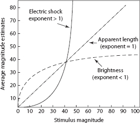
FIGURE 4.7Power-function scales for three stimulus dimensions.

Psychophysical scaling methods are useful in a variety of applied problems. For example, the field of environmental psychophysics uses modified psychophysical techniques to measure a person’s perceived magnitude of stimuli occurring in the living environment. Such analyses can be particularly useful for evaluating the psychological magnitude of noxious stimuli such as high noise levels or odorous pollution. Berglund (1991) and her colleagues developed a procedure that obtains scale values for environmental stimuli from magnitude estimation judgments. With this procedure, the estimates from controlled laboratory studies are used to standardize the judgments people make to environmental stimuli.

Consider, for example, the odor that arises around hog farms (Berglund et al., 1974). They spread wet manure on a field in different ways and, after different amounts of time and from different distances, asked people to judge the magnitude of the odor. The same people provided magnitude estimates for several concentrations of pyridine (which has a pungent odor), and the researchers used these latter estimates to convert the estimates of odor strength for the manure to a master scale on which the scale values for each person were comparable. This sort of analysis provides valuable information about factors that reduce the perceived magnitude of noxious environmental stimuli, in this case how manure is spread and how far the hog farm is away from the people affected by it.

Psychophysical scaling methods have been applied to problems in manual lifting tasks (Snook, 1999). People are able to judge relatively accurately the highest acceptable workload they could maintain for a given period of time (say, an 8-hour work day) based on their perceived exertion under different physiological and biomechanical stresses. So, a package handler’s estimate of the effort required to load packages of a particular weight at a particular rate under particular temperature conditions can be used to establish limits on acceptable materials handling procedures. Comprehensive manual handling guidelines, including the National Institute for Occupational Safety and Health (NIOSH) lifting equation (Lu, Waters, Krieg, & Werren, 2014), described in Chapter 17, have been developed based primarily on studies using variants of the psychophysical scaling methods described in this section.

For a final example, Kvälseth (1980) proposed that magnitude estimation could be profitably applied to evaluation of the factors influencing the implementation of ergonomics programs in industry. He asked employees of several firms to estimate the importance of 21 factors for the implementation of an appropriate ergonomics program in their company. They rated one factor first (say, accident rates) and then rated all other factors according to the ratio of importance relative to the first (e.g., if the second factor was twice as important as the first, they were to assign it a numerical value twice that of the first). Kvälseth’s procedure demonstrated that, surprisingly, the two factors judged to be most important were management’s perception of the need for ergonomic implementation and management’s knowledge of the potential benefits of having satisfactory working conditions and environment. This result was surprising, because these factors were perceived as more than twice as important as the factor that was ranked 12th: the extent of work accidents and incidents of damage to health in the firm.

CHRONOMETRIC METHODS

The rise of the information-processing approach coincided with increased use of reaction time and related chronometric measures to explore and evaluate human performance (Lachman, Lachman, & Butterfield, 1979; Medina, Wong, Díaz, & Colonius, 2015). In a reaction-time task, a person is asked to make a response to a stimulus as quickly as possible. Whereas in the psychophysical approach, response frequency was the dependent variable upon which performance was evaluated, in the chronometric approach we look at changes in the reaction times under different response conditions.

There are three types of reaction-time tasks. In simple reaction time, a single response is made whenever any stimulus event occurs. That is, the response can be executed as soon as a stimulus event (e.g., the appearance of a letter) is detected. It does not matter what the stimulus is. A go–no go reaction time is obtained for situations in which a single response is to be executed to only some subset of the possible stimulus events. For example, the task may involve responding when the letter A occurs but not when the letter B occurs. Thus, the go–no go task requires discrimination among possible stimuli. Finally, choice reaction time refers to situations in which more than one response can be made, and the correct response depends on the stimulus that occurs. Using the preceding example, this would correspond to designating one response for the letter A and another response for the letter B. Thus, the choice task requires not only deciding what each stimulus is, but also that the correct response be selected for each stimulus.

SUBTRACTIVE LOGIC

Donders (1868/1969) used the three kinds of reaction tasks in what has come to be called subtractive logic. Figure 4.8 illustrates this logic. Recall from Chapter 1 that Donders wanted to measure the time that it took to perform each unique component of each reaction task. Donders assumed that the simple reaction (a type A reaction in his terminology) involved only the time to detect the stimulus and execute the response. The go–no go reaction (type C) required an additional process of identification of the stimulus, and the choice reaction (type B) included still another process, response selection. Donders argued that the time for the identification process could be found by subtracting the type A reaction time from the type C. Similarly, the difference between B and C should be the time for the response-selection process.

FIGURE 4.8The subtractive logic applied to simple (A-reaction), go-no go (C-reaction), and choice (B-reaction) reaction times.

Subtractive logic is a way of estimating the time required for particular mental operations in many different kinds of tasks. The general idea is that whenever a task variation can be conceived as involving all the processes of another task, plus something else, the difference in reaction time for the two tasks can be taken as reflecting the time to perform the “something else.” One of the clearest applications of the subtractive logic appears in studies of mental rotation. In such tasks, two geometric forms are presented that must be judged as same or different. One form is rotated relative to the other, either in depth or in the picture plane (see Figure 4.9). For same responses, reaction time is a linearly increasing function of the amount of rotation. This linear function has been interpreted as indicating that people mentally rotate one of the stimuli into the same orientation as the other before making the same–different judgment. The rate of mental rotation can then be estimated from the slope of the function. For the conditions shown in Figure 4.9, each additional deviation of 20° between the orientations of the two stimuli adds approximately 400 ms to the reaction time, and the rotation time is roughly 20 ms/degree. This is an example of the subtractive logic in that the judgments are assumed to involve the same processes except for rotation. Thus, the difference between the reaction times to pairs rotated 20° and pairs with no rotation is assumed to reflect the time to rotate the forms into alignment.

FIGURE 4.9Mental rotation stimuli (upper panel) and results (lower panel) for rotation (a) in the picture plane and (b) in depth.

ADDITIVE-FACTORS LOGIC

Another popular method uses an additive-factors logic (Sternberg, 1969). The importance of the additive-factors logic is that it is a technique for identifying the underlying processing stages. Thus, whereas the subtractive logic requires that you assume what the processes are and then estimate their times, additive-factors logic provides evidence about how these processes are organized.

In the additive-factors approach, we assume that processing occurs in a series of discrete stages. Each stage runs to completion before providing input to the next stage. If an experimental variable affects the duration of one processing stage, differences in reaction time will reflect the relative duration of this stage. For example, if a stimulus-encoding stage is slowed by degrading the stimulus, then the time for this processing stage will increase, but the durations of the other stages should be unaffected. Importantly, if a second experimental variable affects a different stage, such as response selection, that variable will influence only the duration of that stage. Because the two variables independently affect different stages, their effects on reaction time should be additive. That is, when an analysis of variance is performed, there should be no interaction between the two variables. If the variables interact, then they must be affecting the same stage (Schweickert, Fisher, & Goldstein, 2010).

The basic idea behind additive-factors logic is that through careful selection of variables, it should be possible to determine the underlying processing stages from the patterns of interactions and additive effects that are obtained. Sternberg (1969) applied this logic to examinations of memory search tasks, in which people are given a memory set of items (letters, digits, or the like), followed by a target item. The people must decide whether or not the target is in the memory set. Sternberg was able to show that the size of the memory set has additive effects with variables that should influence target identification, response selection, and response execution. From these findings, he argued for the existence of a stage of processing in which the memory set is searched for a target, and that this stage was arranged serially and was independent of all other processing stages.

We can find fault with both the additive-factors and subtractive logics, for several reasons (Pachella, 1974). An assumption underlying both the subtractive and additive-factors logics is that human information processing occurs in a series of discrete stages, each with constant output. Because of the highly parallel nature of the brain, this assumption is an oversimplification that is difficult to justify in many circumstances. Another limitation of these approaches is that they rely on analyses of reaction time only, without consideration of error rates. This can make it difficult to apply these techniques to real human performance problems, because people make errors in most situations, and it is possible to trade speed of responding for accuracy, as described in the next section. Despite these and other limitations, the additive-factors and subtractive methods have proved to be robust and useful (Sanders, 1998).

CONTINUOUS INFORMATION ACCUMULATION

In recent years, researchers have advocated more continuous models of information processing in which many operations are performed simultaneously (Heathcote & Hayes, 2012). Information is not transmitted in chunks or discrete packets, as in the subtractive/additive-factors logics, but instead flows through the processing system like water soaking through a sponge. An important aspect of these kinds of theories is that partial information about the response that should be made to a particular stimulus can begin to arrive at the response-selection stage very early in processing, resulting in “priming” or the partial activation of different responses (Eriksen & Schultz, 1979; McClelland, 1979; Servant, White, Montagnini, & Burle, 2015). This idea has found a good deal of empirical support. Coles et al. (1985) demonstrated empirically that responses show partial activation during processing of the stimulus information in some circumstances. Neurophysiological evidence also suggests that information accumulates gradually over time until a response is made (Schall & Thompson, 1999).

In reaction-time tasks, because people are trying to make responses quickly, those responses are sometimes wrong. This fact, along with the evidence that responses can be partially activated or primed, has led to the development of processing models in which the state of the human processing system changes continuously over time. Such models account for the relation between speed and accuracy through changes in response criteria and rates of accumulation.

One way that we can characterize gradual accumulation of information is with a random walk (Klauer, 2014; see Figure 4.10, top panel). Suppose that a listener’s task is to decide which of two letters (A or B) was presented over headphones. At the time that a letter (suppose it is “A”) is read to the listener, evidence begins to accumulate toward one response or the other. When this evidence reaches a critical amount, shown as the dashed lines in Figure 4.10, a response can be made. If evidence reaches the top boundary, marked “A” in Figure 4.10, an “A” response is made. If evidence reaches the bottom boundary, marked “B,” a “B” response can be made. The time required to accumulate the evidence required to reach one of the two boundaries determines the reaction time.

FIGURE 4.10The random walk model and its relation to speed and accuracy. Information accumulates to the criterion level for response (A) or (B). The relation between the right and left panels demonstrates a tradeoff between speed and accuracy.

Suppose now that we tell the listener that he must respond much more quickly. This means that he will not be able to use as much information, because it takes time to accumulate it. So he sets his criteria closer together, as shown in the bottom panel of Figure 4.10. Less information is now required for each response, and, as a consequence, responses can be made very quickly. However, chance variations in the accumulation process make it more likely that the response will be wrong. As shown in the bottom panel of Figure 4.10, the decreased criteria result in an erroneous “B” response because of a brief negative “blip” in the accumulation process.

Accumulation models like the random walk are the only models that naturally explain the relation between speed and accuracy. Because the models can explain a wide range of phenomena involving both speed and accuracy more detailed quantitative accounts of specific aspects, they provide the most complete accounts of human performance. Another closely related family of models that is well suited for modeling information accumulation assumes the simultaneous activation of many processes. These models are called artificial neural networks, and they have been widely applied to problems in human performance, as well as any number of medical and industrial situations requiring diagnosis and classification (O’Reilly & Munakata, 2003; Rumelhart & McClelland, 1986).

In such networks, information processing takes place through the interactions of many elementary units that resemble neurons in the human brain. Units are arranged in layers, with excitatory and inhibitory connections extending to other layers. The information required to perform a particular task is distributed across the network in the form of a pattern of activation: Some units are turned on and others are turned off. Network models have been useful in robotics and machine pattern recognition. In psychology, they can provide an intriguing, possibly more neurophysiologically valid, alternative to traditional information-processing models. We can describe the dynamic behavior of many kinds of artificial networks by accumulation processes like the random walk, which makes the accumulator models doubly useful.

PSYCHOPHYSIOLOGICAL MEASURES

Psychophysiological methods measure physiological responses that are reliably correlated with certain psychological events. These kinds of measurements can greatly enhance the interpretation of human performance provided by chronometric methods (Luck, 2014; Rugg & Coles, 1995). One very important technique is the measurement of event-related potentials (ERPs) that appear on an electroencephalogram (EEG).

The living brain exhibits fluctuations in voltage produced by the electrochemical reactions of neurons. These voltage fluctuations are “brain waves,” which are measured by an EEG. Technicians place electrodes precisely on a person’s scalp, over particular brain areas, and the EEG continuously records the voltage from these areas over time. If the person sees a stimulus that requires a response, characteristic voltage patterns, ERPs, appear on the EEG. The “event” in the ERP is the stimulus. The “potential” is the change in the voltage observed in a particular location at a particular time.

An ERP can be positive or negative, depending on the direction of the voltage change. They are also identified by the time at which they are observed after the presentation of a stimulus. One frequently measured ERP is the P300, a positive fluctuation that appears approximately 300 ms after a stimulus is presented. We observe the P300 when a target stimulus is presented in a stream of irrelevant stimuli, and so it has been associated with processes involving recognition and attention.

An ERP like the P300 is a physiological response to a certain kind of stimulus. Reliable physiological indices like this are invaluable for studying human behavior and testing different theories about how information is processed. By examining how these measures change for different tasks and where in the brain they are produced, we have learned a great deal about how the brain functions. We can also use these kinds of measures to pinpoint how specific tasks are performed and determine how performance can be improved.

The EEG has been used to study performance for many years, but it has its shortcomings. The brain waves measured by the EEG are like the ripples on a pond: If we throw a tire into the pond, we will reliably detect a change at some point on the surface of the pond. Each time we throw in a tire, we will record approximately the same change at approximately the same time. But if we don’t know for certain what was thrown into the pond and exactly where, the measurement of the ripple will only be able to suggest what happened and where. More recent technology has given us virtual windows on the brain by mapping where changes in neural activity occur. Methods such as PET and functional magnetic resonance imaging (fMRI) measure changes in the amount of oxygenated blood being used by different parts of the brain (Huettel, Song, & McCarthy, 2014). Neural activity requires oxygen, and the most active regions of the brain will require the most oxygen. Mapping where in the brain the oxygen is being used for a particular task provides a precise map of where processing is localized. Compared with the EEG, these methods have very high spatial resolution.

However, unlike the EEG, PET and fMRI have very low temporal resolution. Returning to the pond analogy, these methods tell us exactly where something was thrown into the pond but they are unable to tell us when. The EEG can tell us precisely when something is happening but not what it is. The problem is that PET and fMRI depend on the flow of blood into different brain areas: It takes at least a few seconds for blood to move around to where it’s needed. It also takes some time for the oxygen to be extracted, which is the activity that PET and fMRI record. To test theories about mental processing that occurs in a matter of milliseconds, imaging studies require sometimes elaborate control conditions. Relying heavily on logic similar to Donders’ subtractive logic, control conditions are devised that include all the information-processing steps except the one of interest (Poldrack, 2010). The patterns of blood flow during the control conditions are subtracted from the patterns of blood flow during the task of interest. The result is an image of the brain in which the activity is concentrated in those areas responsible for executing the task.

Like the other methods we have presented in this chapter, psychophysiological measures come with a number of problems that make interpretation of results difficult. However, they are invaluable tools for determining brain function and the specific kinds of processing that take place during reaction tasks. Although the human factors specialist may not always have access to the equipment necessary to record psychophysiological measures of human performance, basic research with these techniques provides an important foundation for applied work. Moreover, work on cognitive neuroscience is being integrated closely with human factors issues in the emerging approach that is called neuroergonomics (Johnson & Proctor, 2013) and in the study of augmented cognition (Stanney, Winslow, Hale, & Schmorrow, 2015). The goal of this work is to monitor neurophysiological indexes of mental and physical functions to adapt interfaces and work demands dynamically to the changing states of the person being monitored.

SUMMARY

The human information-processing approach views the human as a system through which information flows. As with any other system, we can analyze human performance in terms of subsystem components and the performance of those components. We infer the nature and organization of these subsystems from behavioral measures, such as response accuracy and reaction time, collected from people when they perform different tasks. General distinctions among perceptual, cognitive, and action subsystems provide a framework for organizing our basic knowledge of human performance and relating this knowledge to applied human factors issues.

There are many specific methods for analyzing the human information-processing system. We use response accuracy, collected using classical threshold techniques and signal-detection methods, to evaluate basic sensory sensitivities and response biases. We use reaction times and psychophysiological measures to clarify the nature of the underlying processing stages. We can use continuous models of information processing to characterize the relations between speed and accuracy of performance across many task situations.

The chapters in this book report many studies on human performance. The data upon which certain theories are based and recommendations for optimizing performance are made were collected using the methods described in this chapter. When you read about these studies, you will notice that we do not usually provide specific details about the experimental methods that were used. However, you should be able to determine such things as whether the reported data are thresholds, whether a conclusion is based on additive-factors logic, or which methods would be most appropriate in that particular situation. Because the distinction between perception, cognition, and action subsystems provides a convenient way to organize our knowledge of human performance, the next three sections of the book will examine each of these subsystems in turn. In the final section, we will discuss the influence of the physical and social environment on human information processing.

RECOMMENDED READINGS

Eyesenk, M. W., & Keane, M. T. (2010). Cognitive Psychology: A Student’s Handbook (6th ed.). New York: Psychology Press.

Gazzaniga, M. S., Ivry, R. B., & Mangun, G. R. (2014). Cognitive Neuroscience (4th ed.). New York: W. W. Norton.

Gescheider, G. A. (1997). Psychophysics: The Fundamentals (3rd ed.). Mahwah, NJ: Erlbaum.

Lachman, R., Lachman, J. L., & Butterfield, E. C. (1979). Cognitive Psychology and Information Processing: An Introduction. Hillsdale, NJ: Erlbaum.

Luce, R. D. (1986). Response Times: Their Role in Inferring Elementary Mental Organization. New York: Oxford University Press.

MacMillan, N. A., & Creelman, C. D. (2005). Detection Theory: A User’s Guide. Mahwah, NJ: Erlbaum.

Marks, L. E., & Gescheider, G. A. (2002). Psychophysical scaling. In H. Pashler & J. Wixted (Eds.), Stevens’ Handbook of Experimental Psychology (3rd ed.), 4: Methodology in Experimental Psychology (pp. 91–138). Hoboken, NJ: Wiley.

Rosenbaum, D. A. (2014). It’s a Jungle in There: How Competition and Cooperation in the Brain Shape the Mind. New York: Oxford University Press.