
Performance Variables and Model Development
Contents
What are Performance Variables?
Reasons for Creating Performance Variables
What If No Pattern is Reliably Available?
Benefit of Using Performance Variables
Creating Performance Variables
Designing Performance Variables
Model and Characteristics in Predictive Modeling
Now that we have seen where analytics fits in the Information Continuum and how it can be used to solve a wide variety of business problems, we will move into more specific pieces of input variables, models, and then subsequently the decision strategies. The heart of analytics is the algorithm that takes variables as input and generates a model. The first main section of this chapter will walk you through what variables are, how they are built, how good ones are separated from bad ones, and what role they play in tuning models. The second main section will cover model building, validating, and tuning. The chapter concludes with a discussion of champion–challenger models.
Performance Variables
There are a lot of different ways to define variables in an analytics solution. Before we jump into an in-depth discussion about performance variables, Table 4.1 defines the terminology to help you put it in context with what is being used in the marketplace by software vendors, publications, and consultants.
Table 4.1
| Terminology | Definition |
| Columns or data fields | Columns in a database table or fields on a display screen form. Multiple fields make up a record. |
| Variables | Columns or data fields that become candidates for use in a model and are run through data analysis to see which ones will get selected. |
| Performance variables | Aggregate or summary variables built from source data fields or columns using additional aggregation business rules. They also go through the data analysis once they are built to select for potential use in the model. |
| Input variables | These are the variables and performance variables selected for the model as input into the analytics algorithm. This term can refer to both variables and performance variables at times. |
| Characteristics | Input variables combined with their relative weights and probabilities in the overall model. This term is typically used when explaining or describing a model to business users who will be relying on the outcome of the model to make business decisions. |
What are Performance Variables?
Training records are passed through an analytics algorithm to build a model. Each record is made up of input variables. The model is then deployed and new records are passed so the model can provide a resultant. These records have the same input variables as the training set. Figure 4.1 is the example used in Chapter 1 where we had four input variables—age, income, student, and credit rating—and the predictive model was supposed to learn the relative impact of each input variable onto the prediction about a computer purchase.

The classification algorithm (decision trees) used in this case built a tree with the input variables with highest discriminatory power at the top of the tree and then subsequent variables in branches underneath, leading to a leaf of the tree that has a Yes or No as shown in Figure 4.2.

The data (input variables and historical records) is coming from a sales system that tracks the sales of computers and also records some customer information. There is a limit to how many types of variables are stored in the system. Even if the system is designed to handle a lot of information on a sales record, it is usually not properly filled in. Therefore, there can be a situation where the decision tree cannot be built. There are two possible reasons for this:
1. Not enough historical data records available to learn from.
2. The input variables identified do not have discriminatory power between the outcome values.
The first reason occurs when a sales system doesn’t track the lost sales or the customers who didn’t buy. If there are no records with the outcome No (the 0 records), it is not possible for the model to be trained for No and it cannot differentiate between Yes and No. Another case could be that the relative proportion of No is so small that it is not enough to build patterns against the dominant Yes (the 1 records) outcomes.
The second reason occurs when input variables are the same values for both 1 and 0 records. For example, 60–70% of the data for both 1 and 0 records of the data set have the same values for age range, or most of the customers have their input variable as Male for gender regardless if they bought or not. In these cases, the algorithm will discard age and gender as input variables because they have low discriminatory value. Here is a detailed example to explain the reasons why performance variables are essential for a model to perform well.
Reasons for Creating Performance Variables
Suppose a firm ABC Computers sells computers online. They have an order management system that takes orders online, over the phone and fax, as well as through email. The order management system has the data fields shown in Table 4.2 available in its database.
Table 4.2
| Entity | Available Data Fields |
| Customer | Name, address, credit score, age, income, repeat customer, profession, education level, budget, business or personal, marital status, presence of children, promotions, coupons sent, credit rating, etc. |
| Product | Product ID, product type, class, weight, screen size, processor, memory, hard disk, other specifications, price, lot, manufactured date, Mac, PC, etc. |
| Sales channel | Channel ID, channel category, channel partner, channel cost, etc. |
| Sales transaction | Transaction ID, transaction code, timestamp, channel, product, customer, price, payment method, discount, coupon, transaction amount, etc. |
Regardless of how much depth a system has in its design to capture all sorts of relevant data, we know that reality is different, and customers want to provide minimal information while the sales people focus on closing the sale instead of recording data. Here is what data analysis will show if we have a few years of sales data recorded in this system:
■ A lot of the data fields on various records will be empty.
Let’s define a rule of thumb as an illustrative data profile of this sales system. Let’s assume the total number of fields sourced is 70:
■ Total number of fields available: 70
■ Fields mostly with null values: 23 (roughly one-third will usually be empty)
■ Out of 47, fields with good data: 24 (roughly half of remaining fields will have quality problems)
■ Variables available as input variables for the model will be 24 (i.e., one-third of the original field count)
These 24 variables will now be put through a second set of tests to assess their viability as input variables. This is done to make sure the good-quality data filled out has some diversity. So if the field has the same values for all customers who bought and ones who didn’t buy, the fields will not be useful. For example, a field with gender has two possible values, M and F, but if all customers who bought and the ones who didn’t buy were M, this field is of no use. It is entirely possible to lose another 10 or so fields, leaving us with 14 input variables. Let’s assume we have a minimum of two years of data available. If we don’t have enough historical data available we have to stop. But how much data is enough? It is very difficult to answer this question generically without understanding the specific business scenario, however; here is another rule of thumb (with no scientific basis) as a guideline or at least a starting point to work with. If the total business transactions activity where the model is being built is 100 in a calendar year, make sure 40 transactions over the last 12 months are available.
Now when we try to build the model by passing the training set through the decision tree algorithm, the algorithm will try to look at combinations of the 14 input variables and their various values, and will try to find patterns that can reliably distinguish between the 1 and 0 records (respectively, yes or no in this case), meaning customers who bought and customers who didn’t buy.
What If No Pattern is Reliably Available?
This is very important to understand, because this is the inherent nature of analytics. You may not find a pattern that gives you actionable insight. So the entire exercise of data collection, preparation, cost of hardware and analytics algorithm, and human hours—all of that went to waste? This is entirely possible if proper planning is not undertaken beforehand. You may end up without a model or a model with weak performance (more on that later) to show for all the analytics investment. Performance variables come to the rescue in these types of situations. Performance variables are aggregate variables built using historical and trending data, and they are built at the same level of grain as the remaining input variables. In our example, one record of training data represents one customer who had either bought or had not bought a computer. So if some customers had prior sales transactions in the system, a performance variable will be built at the customer record level to capture the previous sales. Table 4.3 shows some examples of performance variables in the context of our computer sales example.
Table 4.3
Performance Variables for Computer Sales Example
| Performance Variable | Data Type | Definition |
| Purchased_in_last_12_mo (more variables can be created for 6 months, 18 months, etc.) | Char(1) | Set to 1 if there is at least one sales transaction for the same customer in the last 12 months; set to 0 otherwise. |
| No_of_visits_online | Number | Pull data from the website to see if visits of the customer can be tracked and counted. |
| No_of_cust_srvc_contacts | Number | Pull data from CRM system to count prior service or sales enquiry calls. |
| 1st_ever_purchase_date | Date | What is oldest purchase transaction date? |
| Last_purchase_date | Date | What is the last purchase date? |
As you can see from the table, there is no end to the creativity or possibilities of how new performance variables can be built. So let’s say the original 14 input variables didn’t result in a good model. We add the 5 performance variables from Table 4.3 and now we have additional input variables that may be able to come up with a strong pattern that indicates BUY = Yes and another strong pattern that indicates BUY = No. If these 5 performance variables don’t yield good results, go back to the drawing board, analyze the data again using traditional reporting and drilling methods, and see what else can come in handy. Tap into other systems, such as warranty or manufacturing systems, to track the parts and suppliers and build aggregate performance variables using additional data, and run the model again until desired results are achieved.
Benefit of Using Performance Variables
Performance variables are a very important aspect of the analytics solution that can save the investment of an analytics project. Creative use of available data and business knowledge should be employed in constantly finding new and interesting performance variables and then test the performance of the model.
1. Even if desired results are achieved, the performance variables should continue to be designed and models built and tested as an ongoing tuning and model improvement exercise.
2. If prebuilt models are purchased for a specific task, they can be kept from getting stale and irrelevant by adding new performance variables to them.
3. If the software investment included a prebuilt model as well as an analytics algorithm like a neural network or decision tree, then the internal team can keep creating newer and more efficient models and yield long-term benefits from the investment in the software.
4. As business evolves, removing some input variables and adding newer performance variables ensures the model predictions are reflective of changing business dynamics. For example, adding online activity– or social media activity–related performance variables to a customer or product profile can be very helpful to incorporate the impact of those channels.
5. In situations where lines of business or categories of products and customer segments are essential in the business dynamic, it may be worthwhile to get a specialist consulting firm to build a baseline model and then use performance variables to create additional models from that for other lines of business or other customer segments.
6. Performance variables allow for the adoption of industry best practices but then provide an added competitive edge in building superior models above and beyond what the competition has. Data from the same ERP system, for example, can be put through a rigorous and innovative performance variables design activity to add more value into the analytics models.
Creating Performance Variables
While good performance variables can significantly enhance a model’s performance, poorly built ones can be detrimental to the analytics exercise overall. It is, therefore, important to carefully consider the following principles while creating new performance variables.
Grain
In the examples in Chapter 3, we emphasized the importance of grain and identified the grain in each example. Grain is the level of detail at which the analytics algorithm will work. An analytics algorithm cannot work at varying grains without some data preparation (ETL) effort bringing it to the same grain. In a clustering example, if we had some points representing customers and some representing households, the intermixed cluster would not make any sense, as the variables used for “likeness” would be different at the household level (e.g., there cannot be one gender representing a household). The grain is tied to the problem statement, and reading the problem statement can explain what the grain is. Similarly, if the problem statement suggests multiple grains, then it needs to be revisited and further refined until one grain is identified.
Range
The range of the performance variables refers to the possible values in a performance variable. Let’s look at a performance variable age_of_position, which represents the aging of a certain type of security that a trader is holding and it is recorded in days and updated every day. The age_of_position can have a range of values from 1 to N. This is called a continuous variable. A variable that has potentially a very large set of possible values and the range of values that may occur on a record is not constrained by any business rule, then it is a continuous variable. The possible values assessment has to come from source system analysis where the data for the variable comes from. If the source system does not put any restrictions on what possible values it can take on, then in theory it can take on any number of unique values, and therefore it is continuous. Continuous variables are not good performance variables and should be avoided if possible. Later in this chapter we will cover how to convert continuous variables into discrete variables.
Spread
The spread of a variable refers to how the population (the entire record set or sample being considered for model creation) is broken out on particular values of the variable. This is the frequency of each value of the performance variable. Let’s use an example to explain this.
Suppose we are building a predictive model that predicts the likelihood of an insurance policy to redeem a claim. As part of that predictive model we designed a performance variable representing the customer profitability that stores the amount of money the insurance company has made on that customer since the inception of the policy. The performance variable has the following details:
■ Name of the performance variable: CUST_PROFIT_LTD_AMT
■ Descriptive name: Customer profitability life-to-date amount
■ Data type: Decimal with length 18 and precision 4 (i.e., up to four decimal places)
The value range is determined by performing the minimum and maximum functions on the performance variable when it has been calculated for all the customers. Now let’s say the total number of customers is 10,000 and we have their CUST_PROFIT_LTD_AMT values calculated. This would be a continuous variable because there is no business rule or restraint on what can be the possible profitability of a customer. A continuous variable will usually have a very sparse frequency chart because each individual unique value may have a very small number of customers. Therefore, the frequency would be 1 or 2 for most of the values. This is not a good spread for a performance variable. Similarly, if most of the population is skewed within a handful of values and the other possible values hardly have any population, that is bad as well. Good performance variables should have a good even distribution.
Designing Performance Variables
The design of performance variables uses the following techniques to convert detailed data into useful performance variables. These techniques can be used in any of the four analytics methods we have covered in the book.
Discrete versus Continuous
As explained earlier in this chapter, continuous variables are not good for analytics models to learn from and assign appropriate weights. Therefore, continuous variables have to be converted into discrete variables with a finite and small manageable set of potential values. The way to do this for numeric values is to build ranges of values and assign them codes. Table 4.4 provides an example.

The right two columns show a discrete set of ranges that should cover the data set of the left two columns. The design question becomes: How many buckets should be built and what should be their ranges? In this example, we have built five buckets that are 200 points apart. This should not be an arbitrary process of coming up with any number of buckets with any range of values in each. If we draw a bar graph for the two columns on the right, we get what is shown in Figure 4.3. The bar graph should be consistent for the distribution of the population within each range. So the desire is to create a graph like the one shown in Figure 4.4.
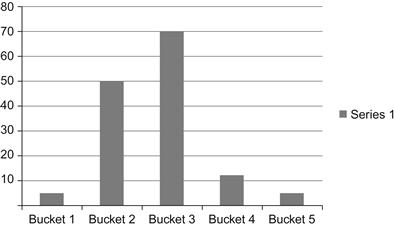

The population is distributed more equally across the values in Figure 4.4. The Frequency function within Excel is a great help in figuring out the value ranges. Each bucket represents a range of continuous values from the original variable. The new variable should be labeled something meaningful to represent the underlying data and its grouping. The buckets can also be coded, meaning a rank or code is assigned to each of them. The ETL process within the analytics datamart will be responsible for building this variable once the ranges have been programmed into the ETL logic. It is entirely possible that in certain situations it is not possible to find such ranges that can evenly distribute the population. In those cases, just use an 80/20 rule to make sure at least 80% of the data to be used in the model training is distributed according to the chart in Figure 4.4.
For other types of continuous data like addresses, try using cities or zip codes to group them in a finite set of manageable values. Strings-based values are almost always continuous, and it is very difficult to convert them into a discrete set of values. The only available option is to convert them into some kind of a higher grouping with a code representing several continuous values.
Nominal versus Ordinal
Another design principle to consider while building performance variables is nominal values versus ordinal values. Ordinal values have an inherent order in the values, so a value of 100 and a value of 200 would imply that the second value is of higher order than the first. Nominal values mean there is no inherent relationship between the values, therefore 100 should be treated the same as 200. When building discrete value sets for continuous data, care should be taken not to create ordinal values or make sure the data mining software has a parameter that can be set to not treat the values as ordinal.
Atomic versus Aggregate
Atomic data or input variables as described earlier in the chapter typically do not fall into the performance variable definition as performance variables are built from atomic variables. They are summaries, intervals, ratios, etc., but are typically not readily available in operational systems.
Working Example
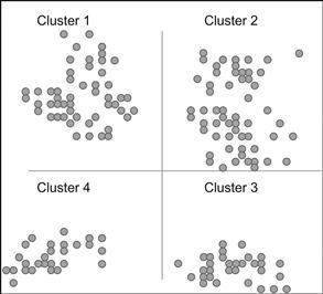
As described in Chapter 3, the art and science of analytics come together at the performance variable level. To understand their impact on the performance of an analytics model we have to be clear on the definition of grain. Analytics algorithms may be K-means algorithms for clustering, regression or neural network algorithms for prediction, or optimization or forecasting algorithms. They work with millions and millions of records at the same grain, meaning all records represent the same entity. For example, one record represents one customer or one record represents one account. They cannot work with one record being a customer and another being an account. So if we are trying to segment our customers into clusters, it would mean that the input data to the algorithm will be one point plotted per customer. Figure 4.5 shows an example of clustering to explain the concept of grain.

Each point represents one customer record with several variables, and the values of those variables have been resolved to result in one point. After plotting them, the clustering algorithm goes through numerous iterations to start to build clusters out of this scatter. The end state looks something like Figure 4.6 where the algorithm puts them into clusters and labels them. In this process one dot represents one customer and therefore it is at the customer grain. If we were using only one variable in the customer record, let’s say customer ID, the algorithm would not be able to find any similarities to bring the dots closer, and the end state of the model would still be the same scatter plot and the tool would probably label it as cluster 1. Therefore, the entire customer population would become one cluster, rendering the effort useless.
For the algorithm to figure out the “likeness” in these dots or points in a multidimensional Euclidean plane, it needs more than just the customer ID to establish likeness. Let’s say we add two more variables, age and gender, into the record and try again. If our customer base is more or less in the same age range—for example, a sports drink manufacturer will have the majority of their customers in the 17–37 age range and may be skewed in favor of males at 78% and females at 22%—then the algorithm will still struggle to find multiple clusters. It may find just three to four clusters with each having millions of customers, still rendering it useless for any effective campaigning. Increasing the variables will help ensure the variables are not skewed toward certain values within their range. But adding too many variables may contribute to losing likeness and very small clusters of 10–15 customers may end up clustered with some very large ones. So the variables, their value spread, and their ability to dissect the population are central to getting the clustering algorithm to produce good results. It is important to note that the same clustering algorithm is being used, but the variables and their quality are determining the quality of output from the model.
Using this as the premise, if we are to add interesting variables, since one point can only have one customer, those additional variables have to be at the customer record level. So a variable like Popular_Products_Purchased that can have multiple values per customer cannot be built just like that. It will have to be transposed to act like columns on a customer record and therefore limit it to a handful of popular products (maybe three or five). So the customer record will get three columns: POP_PROD_PURCHASE_1, POP_PROD_PURCHASE_2, and POP_PROD_PURCHASE_3. These are called performance variables since they exist in a different grain of data, but they have to be built to bring them to the grain of the record where the analytics algorithm is being applied. The definition of “popular” has to be agreed on and programmed on the detail-level data and then pick the top three that become performance variables.
Performance variables are needed because they can spread the data in a good mix that allows the algorithms to produce better results. This is why interesting variables can create very powerful models.
Model Development
An analytics model is the heart of an analytics solution, as it is responsible for producing the desired output. The better the model is, the better the value of the output for business decisions. This section covers what a model is, what it looks like or what it contains, how to validate its effectiveness so decisions can be made, and finally how to detect the weakness in a model and tuning it accordingly.
What is a Model?
As described in Chapter 1, it is important to differentiate between a model and the algorithm. Data passes through an analytics algorithm to produce a model. The model takes input records and then produces an output (forecasted, descriptive, predictive, or optimized). In this section we focus on descriptive and predictive models only. Forecasting and optimization models in their description and layout are very similar to predictive models and both techniques have been around for a long time. There is also not much of a mysterious fog on the magical powers of forecasting, since there is nothing hidden within a data mining algorithm or software like we have in predictive and descriptive analytics software. As you will see in the following, forecasting models can be a simple linear algebra equation not requiring the explanation needed of a predictive or descriptive model.
Model and Characteristics in Predictive Modeling
If you want to touch and feel a model, in the following example you can find what it would look like once produced. Some software packages do not allow for easy access to this level of detail on a model. There are good reasons for this, because if input and exact weights of characteristics within the model are known, when a model runs, input can be manipulated to get the desired output. Sometimes leaving a model as a black-box may not be a bad idea. Following is an example of a consumer risk model that takes input data from a loan applicant and tries to produce a risk score. A high score indicates lower risk and vice versa.
■ Input variable: Age_range_code
| Value | Weight |
| 17 or below | Policy reject, return zero score |
| 18–24 | 100 |
| 25–45 | 150 |
| 46–62 | 200 |
| 63 and above | 125 |
■ Characteristic 2: Previous loan status
■ Input variable: 12_mth_prev_loan_history_status
| Value | Weight |
| One or more loans and up-to-date payments | 200 |
| No loans before | −50 |
| One loan where two payments have been late in the last 12 months | −100 |
| One loan where one payment was late in the last 12 month but not in the last 6 months | 150 |
| More than one loan and paid successfully in the last 12 months | 250 |
Similarly, this type of detailed definition is available for 12–16 characteristics in a typical risk scorecard. This is one example of what a model looks like, but different software may produce different outputs, visuals, actual mathematical equations, etc.
There are two important concepts here: the maximum weight and the weight distribution across the possible values of the variable. Let’s assume the total score for consumer risk is 1,000; the two variables we looked at had the maximum weight of 200 and 250, meaning they account for 450 out of 1,000, or 45% of the total score. The other variables will account for the remaining 55% of the score. So the first step of building a model is to identify the variables and their relative weights with respect to each other. The discriminatory power of a variable to distinguish good and bad records is used to identify the variables that will play a role in the model—that is, they will become characteristics. As input variables from the training set are converted into characteristics by the algorithm to form the model, the relative weight or importance of the variable also emerges with respect to other characteristics in the model. It can be numeric, as used in the preceding example (regression-based models), or it can have probabilities representing their discriminatory power (decision trees).
Once the relative weight of the characteristic is established within the model, we have something that looks like Table 4.5. Scorecard is a numeric representation of a model.
Table 4.5
| Characteristics | % Weight | Maximum Score |
| Age | 20% | 200 |
| Previous loans | 25% | 250 |
| Income | 15% | 150 |
| Residence | 20% | 200 |
| Marital status | 5% | 50 |
| Education | 15% | 150 |
| Total | 100% | 1,000 |
These are characteristics, and each of them could in itself be a more complex derived or aggregated performance variable. In this example the loan decision is being made on this data from the applicant (and from credit bureaus) to assess the risk. This takes care of the maximum weight that each characteristic gets.
The second concept is that of the weight distribution across the various possible values of each characteristic. That problem is broken down into two pieces: the possible values and the weight of each value. For the age characteristic, we used 5 different possible values:
We could use 6 values or 10 values so why these 5? The rule of thumb for identifying the possible values should follow the same approach as discussed in the “Designing Performance Variables” section. The possible values are tied closely into the distribution of the overall population. Once the values have been identified, the weight distribution is based on what role each value has played in determining the 1 or 0 records—that is, the discriminatory power. Data mining tools identify the weights themselves and provide as an output of the training activity as the model is built.
In regression-based models, this level of detail is abundantly clear—a statistician figures out the variables, their values, and their relative weights. Regression software packages also provide visibility into this level of detail but data mining predictive algorithms may not. It is alright to treat the data mining algorithm and the model it creates as a black-box. This level of detail is needed for tuning models, so if data mining software doesn’t provide the detail, how do we tune the predictive models? We will deal with that later in the “Model Validation and Tuning” section.
Model and Characteristics in Descriptive Modeling
The descriptive models are different in nature from predictive models since they don’t need to perform as accurately as the predictive models need to. Since predictions are for a potential future event and business wants to exploit that knowledge and take actions on the predictions, the reliability of the prediction matters a lot. A descriptive model, on the other hand, is describing the data in a form that allows for future action strategies, but it is not a precise event. Rather, it is a perspective into large quantities of data, so business can make sense of the data. It describes data in clusters or association rules so it doesn’t need to be accurate, just approximate. Descriptive analytics has input variables, but their values and weights function differently. When a descriptive analytics model like clustering is complete or built, here is what you find:
■ Cluster affinity (closeness of one cluster to another on the Euclidean plane)
■ Input variables and their values (or range of values) in each cluster
■ Probabilities and correlations of variables within each cluster
That makes the model and its characteristics in descriptive analytics much simpler to review, understand, and use. In predictive analytics, a future event is predicted and that has to be exploited favorably. The focus is the event and, therefore, the usage is tied to the event as well. In contrast, the descriptive model output is an explanation of the data using a structured form like clustering or social network analysis. Once the output is analyzed the question of exploiting this insight becomes wide open to interpretation and innovation. Therefore, the descriptive model’s output is not expected to meet any fixed criteria. This distinction is further explained in the next section.
Model Validation and Tuning
Model validation is essential because of the black-box nature of machine learning algorithms. Once the algorithm has been acquired and data is run through it to build the model, it is important to know what kind of model was built. Is it reliable? Is it a good model? Can business decisions be made on that model? What happens if the model is wrong? The answers to these questions are more important, since this book is encouraging increased use of data mining to solve problems across all functions of a business. It is unlikely that functions of an organization, from HR to finance to procurement and operations, all have access to people who can mathematically review and validate the models. Depending on the data mining software or package, it may not be possible to fully uncover the workings of the algorithm, reconfigure the settings, and ensure good output, even if data mining experts are available on staff. Therefore, with the spirit of this book, we will present a simplistic method of validating a model to satisfactorily answer the questions just posed.
The model validation for predictive models is more critical than the descriptive models since predictive models directly influence a business transaction. The tuning is simply the process of getting the model to pass the validation test. The validation of analytics models is an approximation based on a benchmark of potential usefulness. If the model’s use is not improving the results within the underlying problem statement, it needs tuning. For example, if a credit card default prediction model assigns “low risk” to customers who keep defaulting, then the model fails the validation. The same is true if the model keeps assigning “high risk” to customers who continue to be good customers. We will look at the predictive model validation first.
Predictive Model Validation
In a predictive model, since an event is being predicted, low False-Positives would imply the model is working. False-Positive is a term used to indicate the error rate of a model’s predictions. A false-positive rate of 15% would imply that of the predictions made, the model was wrong 15% of the time. False-Positive counts both aspects of error in predicting an outcome i.e., when model predicts an event and it doesn’t occur and when model doesn’t predict an event and it does occur. However, if a probabilistic output of the predictive model is being considered on an outcome (estimation), then only high-probability outcomes of an event will qualify as an event and then their false positives will be evaluated. Let’s use an example to explain this.
A shipping and logistics company moves boxes and containers from one location to another. They want to predict which shipments will get delayed. They take a sample set, let’s say the last 12 months of shipping data, and they assign 1 to shipments that were delayed and 0 to shipments that made it on time. They ran 90% of that training data through a decision tree data mining algorithm and a model is built. When they tested the model with the 10% of training data that was set aside, they get a results matrix that looks like the following. Assume that 100,000 records were used in total so the model testing was carried out on 10,000 records while 90,000 were used for training.

■ First inference: The model is 91% accurate for predicting shipments on time (7,840 out of 8,610).
■ Second inference: The model’s accuracy is 155% for predicting delayed shipments, or an error rate of 55% (2,160 instead of 1,390).
However, both inferences are misleading since we do not know the exact count of shipments that were actually delayed and have been predicted to be delayed or on time. So we build another matrix, called a confusion matrix, that shows where the model is actually wrong and where it is correct.

aShows where the model was accurate since the predicted outcome and the actual outcome were the same.
So:
■ The total where the model is correct is 7,670 + 1,220 = 8,890 out of 10,000 (89%).
■ The total where the model made a mistake is 940 + 170 = 1,110 out of 10,000 (11%).
The error rate is 11%, or the accuracy is 89%. The validation or evaluation of a predictive model is a science in itself. There are methods like the Kolmogorov–Smirnov Test (Kirkman, 1996), also known as the KS-Test, and Gini Coefficient (Gini, 1955), among various other methods to compare and evaluate predictive models. Explanation of these methods is out of scope for this book, as this is an introductory text designed for simplifying analytics adoption. The 89% accuracy of the model in our example above, is that good enough? Can the model be put into production? Let’s look at some simple validation approaches.
Validation Approaches: Parallel Run
The simplest approach to evaluate the performance of a predictive model is to compare it to the non-analytics way of doing things. One approach is to randomly make some decisions using the predictive model and the remaining using the current business practices (which may be automated using some expert rules or are subject to manual review). Since we are still validating the model, the decisions that ran through the predictive model can still be reprocessed through the current manual process, but the results of the model should be saved for review in a few months to see if the prediction model results fare better than the manual decisions.
Let’s take an example of a credit application system that has an embedded default prediction model:
■ Input: The applicant’s personal and financial information, credit report, and loan product parameters.
■ Output: Credit risk score; a high score means low risk and a low score means high risk.
■ Decision strategy: If the score is below the cutoff, reject the application.
Let’s say 50% of the applications were processed through a manual process and 50% were processed through the model; the outputs were saved for validation purposes.
Management and business owners typically like this approach because it gives them better comfort and belief in analytics. Even though most of the inner workings are a black-box to them, the results shown in Figure 4.7 will be very transparent and convincing. The downside of this approach is that if the model was weak and didn’t perform as expected and the results were not convincing, the analytics team will have to go back to the drawing board for another attempt at adding more variables or changing the existing ones. Usually there are three to five iterations before a model works satisfactorily, and it will take roughly 12–18 months to adopt a predictive model, as each model will need some quiet period to collect the results.

Figure 4.7 shows the applications that should’ve been rejected according to the model and the applications that should’ve been accepted. If after a few months of observation the manually accepted applications turn out to have defaults, then the model was right.
This approach has a side benefit, that of return-on-investment calculation on the analytics solution. If the money saved from prevention of defaults and the money that could’ve been made on rejected applications (that the model pointed out to be acceptable) added up for say three years is more than the cost of the analytics solution, then we know it is a good investment.
Validation Approaches: Retrospective Processing
In this approach we simply calculate the error rate or false-positive rate of the model from the 10% validation data and review its cost implications. In our shipping and logistics company example, the purpose of the model was better customer experience, retention and repeat business, and reduced fines or penalties when shipping SLAs were missed. If we add the cost of customer churn, lack of repeat business, and fines, that will be the total cost when a quantitative approach is not used. If we use a predictive model for identifying the potentially delayed shipments and prevent that cost from being incurred, we may create an overhead of 11% since the error rate was 11%. If that equation is favorable and makes good business sense, then we should adopt the model, otherwise we should figure out the threshold where the model will make sense and go back to tuning the model using additional or modified performance variables. On the other hand, if an existing practice of predicting the delays is in place using a subjective or nonquantitative method, look at its error rate, and if the predictive model has a better error rate, then the model is validated.
Champion–Challenger: A Culture of Constant Innovation
A champion model is the one in place that helps a business carry out analytical decisions. A challenger model is a fine-tuned version of the same model that is solving the same problem but using a different approach. The difference could be as simple as changing the design of an existing performance variable, such as instead of representing three months historical data for an event, it could represent six months’ worth (TOT_PURCHASE_AMOUNT_LAST_6_MTHS). Or it could be as complicated as taping into an additional data source or changing the algorithm all together (e.g., going from a decision tree to a neural network).
As a guideline, for any model that is in production and actual business decisions are being made using the model, there should be a performance review quarterly or at most semi-annually. When off-the-shelf prepackaged models are purchased, the maintenance and tuning is typically priced separately. That cost should be factored into using analytics models. You either pay in building the internal capability to track and tune the performance of the models or you pay the vendor supplying the model. Skipping on that cost is dangerous, because it will not be known when the model is performing poorly and wrong decisions will be made.
Chapter 6 details how previous versions of the models have to be kept with the decisions performed using those models even when they are retired. How are various generations or versions of the model kept along with various challenger models that never proved better than the champion models? A careful audit trail is required for investigation and analysis when incorrect decisions based on models get highlighted by the business and a review is ordered.
The most important aspect of the champion–challenger constant improvement cycle is how do we know the challenger is better? Use the same technics described previously in this chapter in the “Model Validation and Tuning” section and see if the numbers from the challenger model are better than the champion model. If they are, you can move into promoting the challenger to the champion. However, that would require careful planning and coordination since various cutoffs of scores for decisions may need to be adjusted, and people and processes relying on the numbers from the models have to understand the change is coming.
When the challenger model takes ahold, start working on yet another innovative model using newer forms or newer sources of data and try it out to see the impact. Also track the performance of the model to know when it needs tuning. It is important to differentiate between tuning a model and replacing a model. Tuning is basically adjusting the input variables, while replacing means that a new approach to solving the problem is being considered. For example, on a propensity model where you predict the likelihood of a customer buying using a coupon or responding to a discount offer, you may have used several variables from the sales system and several from the call center and online store. Based on that, the model was built, and when it starts to deteriorate in its performance, you may tweak the variable definitions and add additional definitions. This is tweaking, because the underlying approach is that sales and customer interaction historical data is a good indicator of propensity. However, a challenger model would be where you introduce the human resource system variables. Now the underlying approach to solving the propensity problem is going through a fundamental change, where you are hypothesizing that some employee variables, indicating experience, education, salary, bonus, etc., have some impact on propensity and historical sales. This would be a challenger model.
This distinction is necessary because creating a new model has different cost implications versus tuning a model. There is additional overhead in data sourcing, integrating, identifying metrics, identifying candidate variables, etc. for building a new challenger model.
In Chapter 5, we will deal with how to handle the output of the model and convert it into an automated decision strategy.