Defining Analytics
Contents
Definition 1: Business Value Perspective
Definition 2: Technical Implementation Perspective
The Hype
Analytics is one of the hot topics on today’s technology landscape (also referred as Big Data), although it is somewhat overshadowed by the high-profile social media revolution and perhaps also by the mobile revolution led by Apple Inc., which now includes smartphones, applications, and tablets. Social media, mobile, and tablet revolutions have impacted an individual’s life like never before, but analytics is changing the lives of organizations like never before. The explosion of newer data types generated from all sorts of channels and devices makes a strong argument for organizations to make use of that data for valuable insights. With this demand and emergence of cost-effective computing infrastructure to handle massive amounts of data, the environment is ripe for analytics to take off. However, like any technology that becomes a buzz word, the definition becomes more and more confusing with various vendors, consultants, and trade publications taking a shot at defining the new technology (analytics is actually not new but it has been reborn with Big Data; see Chapter 11). It becomes extremely difficult for people intrigued by this topic to sort through the confusing terminology to understand what it is, how it works, and how they can make use of it. This happened with ERP and e-commerce in the mid- to late 1990s and with CRM in the early 2000s. Over time, as the industry matures, consensus emerges on what is the definition and who are the dominant players, respectable trade publications, established thought leaders, and leading vendors.
The data warehousing industry was the first to tackle data as an asset and it also went through a similar hype cycle where terms like OLAP (online analytical processing), decision support, data warehousing, and business intelligence were all used to define some overlapping concepts with blurring boundaries. The term that eventually took hold is business intelligence (BI) with the data warehouse becoming a critical central piece. BI included everything—activities like data integration, data quality and cleansing, job scheduling and data management, various types of reporting and analytical products, professionals, delivery and maintenance teams, and users involved with getting value out of a data warehouse. BI as an industry has matured and become well structured with accompanying processes, methodologies, training, and certifications, and is now an essential part of IT in all major public or private organizations.
While analytics is an extension of BI in principle and it is natural for existing BI vendors, implementers, and professionals to extend their offering beyond reporting into analytics, it should be separated from a traditional data warehousing and reporting definition. We have lived with that definition of BI for the last 10 years and there is no reason to confuse the landscape. It is important to differentiate between BI in which reporting and data warehousing are incorporated, and analytics in which data mining, statistics, and visualization are used to gain insights into future possibilities. BI answers the question “How did we do?” whereas analytics answers the question “What should we do?” BI answers the question “What has happened?” and analytics answers the question “What can happen?” The temptation to replace BI with analytics as an overarching term to refer to anything related to data is going to be counterproductive. The material presented in this book will provide a detailed step-by-step approach to building analytics solutions and it will use BI as a foundation. Therefore, it is important to keep the two concepts separate and the two terms complimentary.
The Challenge of Definition
To help demystify analytics and provide a simplified view of the subject while looking at its significance, wide use, and application, we will look at several definitions:
■ Merriam-Webster (2012): The method of logical analysis.
■ Oxford Dictionary (2012): The term was adopted in the late 16th century as a noun denoting the branch of logic dealing with analysis, with specific reference to Aristotle’s treatises on logic.
■ Eckerson’s book (2012), which covers the expertise of leading analytics leaders, defines it as everything involved in turning data into insights into action.
These are very broad definitions and don’t really help understand analytics in an implementation and technology context. Instead of defining analytics as a dictionary would do, let’s look at some characteristics of analytics that can help simplify the conceptual foundation to understand its various moving parts, allow filtering of the marketing hype, and look for pieces needed for specific solutions regardless of what they are being called.
We will use two different perspectives to lay out the characteristics of analytics: one is related to how business value is achieved and the other regards how it is implemented. But the definition of analytics here will be more of a definition of analytics solutions overall and not necessarily a few tools or techniques. The definition will be broad enough to help readers understand and apply it to their benefit, yet it will have specific boundaries to distinguish from other related technologies and concepts to ensure expectations are met from analytics investment.
Definition 1: Business Value Perspective
The business value perspective looks at data in motion as it is generated through normal conduct of business. For this data, there are three variations of value: the present, the past, and the future, in that exact order. When data is created, referenced, modified, and deleted during the course of normal business activities, it lives in an operational system. The operational system at any given time can tell us where we stand now and what we are doing now. The data at a specific point in time is of relevance to people in day-to-day operations selling merchandise, reviewing applications, counting inventories, assisting customers, etc. The data and the activities are focused on very short durations from a time perspective. This data from “Now” is the first variation of business value—that of present activities; over time, it becomes stale and is retained for recordkeeping and starts to build history.
This historical data, usually in a data warehouse, can then be reviewed to understand how a business did in the last month, quarter, or year. This information is relevant to business managers since they can see business performance metrics, such as total sales, monthly counts of new customers, total number of service calls attended, total defects reported, total interruptions in business, total losses, etc. This is typically done through reporting. The analysis from this historical review of information provides managers the tools to understand the performance of their departments. This is the second variation of business value—that of past activities. This leads into what the managers should be doing within their departments and business units to improve their performance. The historical data doesn’t tell them what to do; it just tells them how they did. Historical data is then run through some advanced statistics and mathematics to figure out what should be done and where the energies should be focused.
This leads to the third variation of the business value—that of future activities. Analytics (or Big Data) belong to this variation: What should we be doing? Any tools, technologies, or systems that help with that can qualify to be in the analytics space. This business value perspective of analytics is driven from the usage or outcome of the data rather than the implementation. Figure 1.1 explains this definition.

Therefore, the business perspective of the analytics definition deals with future action and any technology, product, or service that contributes towards the action can qualify to be part of analytics solutions. It can be argued that historical analysis also gives ideas on what should be done in the future, such as terminate an unprofitable product line or close down a store, but later chapters will show that the analytics solution is actually very specific about future actions based on historical trends and patterns and is not reliant on humans interpreting the historical results and trying to determine the actions rather subjectively.
Another way to define analytics will be from the technical perspective. This perspective has been influenced from the published works of Thornton May on this topic (May, 2009).
Definition 2: Technical Implementation Perspective
The technical implementation perspective describes the characteristics of analytics in terms of the techniques used to implement the analytics solution. If any of the following four data analysis methods are used, the solution is qualified as an analytics solution:
2. Descriptive analytics (clustering, association rules, etc.)
3. Predictive analytics (classification, regression, and text mining)
These methods will be defined in more detail subsequently in this chapter, but they will be layman’s definitions and will only provide a broad understanding of these methods and their use. For a detailed understanding of these techniques, a lot of good literature is already available in the market like Data Mining Techniques: For Marketing, Sales, and Customer Relationship Management by Gordon Linoff and Michael Berry (2011), and Data Mining: Concepts and Techniques by Jiawei Han and Micheline Kamber (2011).
If the use of these techniques makes it an analytics solution, why not use this definition alone? Why do we even need the first business perspective definition? Data visualization is what throws off this technical definition. Data visualization deals with representing data in a visual form that is easy to understand and follow. Although it is representing the past, once the visual representation emerges, there are always clusters of data points visually obvious that immediately lead to future actions. For example, in case of geographic information systems (GISs; also clubbed in data visualization), the historical sales data is laid out on a map with each point representing a customer address. Immediately looking at the map with clusters of customers in certain areas, management can decide about advertising in that region, opening a store in that region, or increasing the retail presence through distribution. This geographic cluster of customers is very difficult to detect from traditional reporting. Even though the GIS doesn’t use any of the four techniques, it still represents a future actionable perspective of business value.
So why not add visualization to the list of four techniques? It is a subjective argument and open to debate and disagreement. Even though it provides future actionable value, in my view, it is still a reporting mechanism, just more pleasing to the human eye. It is closer to descriptive analytics in definition since it describes the historical data in a visual form, but it is no different than plotting lines, charts, and graphs. Subsequent material (see especially Chapter 5) will illustrate that the implementation of data visualization is very hard to automate and integrate into business operations without a manual intervention looking at the visualization to support automated decisions. Its implementation is also closer to reporting and analytical applications and dashboards rather than, let’s say, a prediction or decision optimization solution.
So basically, an analytics solution, technology, or service is only qualified to be labeled as analytics if it fits either of the two preceding definitions. A more conservative way of sketching the boundaries around analytics would be to use both definitions when labeling something as analytics. Text mining is another anomaly that qualifies on the first definition but fails on the second, yet its solution and implementation is closer to prediction even when it doesn’t use typical predictive techniques.
The next section explains these selective analytics techniques in a little more detail. The rest of the book relies on these definitions to demonstrate the value of analytics, the design of an analytics solution, the team structure and approach for adopting analytics, and the full closed loop of integration of analytics in day-to-day operations through decision strategies.
Analytics Techniques
Again, there are four techniques that we will use to define and explain analytics along with its use, implementation, and value:
2. Descriptive analytics (primarily clustering)
3. Predictive analytics (primarily classification but also regression and text mining)
Each of these is a science crossing computer science, mathematics, and statistics. An analytics solution will use one or more of these techniques on historical data to gain interesting insights into the patterns available within the data and help convert these patterns into decision strategies for actions. Each of these techniques has a particular use and, depending on the goal, a specific technique has to be used. Once the technique has been identified, the methodology, process, human skill, tools and data preparation, implementation, and testing make up the rest of the solution. The internal workings of these techniques are beyond the scope of this book. There are numerous other books available that explain these in greater detail down to the mathematical equations and statistical formulae and methods. For detailed review of these techniques, use any of the following recommended reading:
■ Artificial Intelligence: A Modern Approach (Russell & Norvig, 2009)
■ Artificial Intelligence: The Basics (Warwick, 2011)
■ Data Mining: Practical Machine Learning Tools and Techniques (Witten, Frank & Hall, 2011)
Algorithm versus Analytics Model
It is important to explain the difference between the algorithm and the analytics model in this context of analytics techniques. Each technique is implemented through an algorithm designed by people with PhDs in statistics, mathematics, or artificial intelligence (AI). These algorithms implement the technique. Then a specific problem feeds data to the algorithm, which works like a black-box to build the model; this is called model training. The analytics model is based on the learning gleaned from the training data set provided. The model, therefore, is specific to a problem and the data set used to build it contains the patterns it has found in the input data. The algorithm is a general-purpose piece of software that doesn’t change if the data set is changed, but the model changes with changes in the training data set. Using the same algorithm, let’s say a clustering software can be used to build clusters of retail customers at a national store chain or can be used to build clusters of financial transactions coming from third-party financial intermediaries. The model will be different (i.e., the variables and characteristics of a cluster) with changes in input data, but the algorithm would be the same.
How good a model you can create given an available algorithm is the same as how good a tune you can create given a particular musical instrument. There is no end to possible improvements in building innovative models, even if using the same algorithm (see Chapter 4 for more explanation on this). The analogy between algorithms and musical instruments further extends: a very high-end and expensive acoustic instrument can certainly improve the sound of the tune you have written compared with an inexpensive instrument. The same is true for algorithms, such as:
■ You can get algorithms for free that implement the analytics techniques or ask a PhD student in statistics or AI to build one for you ($).
■ You can get algorithms prebuilt in vendor software applications and databases ($$).
■ You can buy pure-play high-end algorithms from specialized vendors ($$$).
If you pass the same data set through these three options, some improvement in each progressing model’s performance will be evident. But as you cannot create a great sonata by investing in an expensive instrument, an expensive algorithm alone will not result in a quality solution that would deliver business value. Successful application of analytics techniques to business problems requires a lot of other pieces—the algorithm is only one critical part.
The intention of this book is to treat the scientific complexity of a technique and its algorithm as a black-box and explain what they do, what they take as input, what they produce as output, how that output should be used, and where these techniques yield the best value. Readers are not expected to master how to build a new and more robust clustering algorithm, for example, but rather learn how to identify a problem and apply clustering to solve the problem in a methodical and repeatable way. The approach is not very different from a book written about software programming that briefly touches upon the operating system and treats it as a black-box that the programming software interacts with.
Forecasting
Other related terms for forecasting are time series analysis or sequence analysis. While the people spending their lives defining these terms and carrying out years of research and publishing papers on the finer points of these techniques may be appalled at my clubbing all of these within forecasting, my intention is to simplify the concept so it can be understood and used. Forecasting involves looking at data over time and trying to identify the next value (Figure 1.2). Simply put, if the data points or values are plotted on a graph, then identifying the next value and plotting it on the graph is forecasting. The approach used is very similar to the following problem. Suppose you have a series of numbers like 1, 3, 5, 7, 9, and you are asked what the next number would be—11. How did you derive that value? By looking at the pattern common between each value with its predecessor and successor, the same pattern was applied to the last value to determine the next value. This was a very simple case. Now let’s take a little more complex problem. Let’s say a series of numbers is 1, 4, 9, 16, 25—what will be the next value? It would be 36. Here the predecessor-to-successor relationship is not as simple as before, but actually a hidden series of 1, 2, 3, 4, 5, 6 is being squared. These examples illustrate the basic principle of identifying a pattern in a series of values to forecast the next value.

Various algorithms exist to provide forecasting like time series analysis, which is extensively used in business for sales and revenue forecasting. It uses a moving average to identify the next value based on how the average of the entire data set changes with each new value. To understand the complexity involved in forecasting, let’s look at two extreme examples. Weather forecasting (e.g., what will be the high temperature for tomorrow) can be approached simply by putting down the high daily temperature of the last two years, and based on that, predict what will be the temperature tomorrow. This would be one extreme, that of simplicity, as only one variable, daily_high, is being used and plotted on the graph to see what will be the next value, and it may provide a number that may turn out to be fairly reasonable. However, this is not factoring in barometric pressure, a weather system coming from the west, rain or snowfall, effects of carbon emission, cloudy skies, etc. As we add these additional variables to the model, the forecasting cannot be simply done by plotting one variable on a graph and visually plotting the next value; it would require a more complex multivariable model built from a forecasting algorithm. Time series–based forecasting algorithms are usually embedded in database systems or available as code libraries for various programming environments and can be easily incorporated into an application system. They are used by supplying a learning set to the algorithm so a model can be built. Then the model takes input data and produces output value as a forecast.
Descriptive Analytics
Descriptive analytics deals with several techniques, such as clustering, association rules, outlier detection, etc., and its purpose is to look for a more detailed description of the data in a form that can be interpreted in a structured manner, analyzed, and acted on. If an organization has two million customers, any meaningful analysis of these customers would require questions such as:
■ Who are they and how do they interact with the organization?
Answering these questions for two million customers requires some grouping of these customers based on their answers to get anything useful out of the analysis. A lot of times, in the absence of any descriptive analytics technology, the first 100 records will get picked up for further analysis and actions. Descriptive analytics describes using forms and structures that allow analysts to make sense of mountains of data, especially when they are not sure what they may find. This is also known as undirected analytics where data mining algorithms find patterns, clusters, and associations that otherwise may not have been known or even sought.
For further explanation we will use clustering to explain descriptive analytics in a little more detail.
Clustering
Clustering is a method of grouping data points into clusters based on their “likeness” with one another. This method is used widely in customer analytics where customer behavior and demographics are used to see which customers can be grouped together. Marketing campaigns and other sales and service driven promotions are then designed for each cluster that shows similar historical profiles (similar number of purchases, type of products purchased, gender, income, marital status, zip code, etc.) to manage customers consistently. The most popular clustering algorithm is K-means. This algorithm is commercially available in database systems and from third-party companies. It is also available in open source in the R Project (R Foundation, 2012) and through open-source software like WEKA (Group) that is extensively used in academic circles. Figures 1.3 through 1.5 explain how K-means works to build clusters from a collection of data points. Figure 1.3 shows a simple plotting of points in the Cartesian plane.
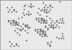


K-means relies on Euclidean distance to start to see which points are closer to each other and brings them closer to form clusters. The idea is a point is closely related to another point that is closer to it rather than to a point that is farther away.
As the algorithm iterates through the plotted points and keeps moving them closer, there comes a time when it can no longer bring the points closer. This is controlled through various parameters that clustering algorithms allow for users to set. At that time, clusters are complete. There can be some points or smaller groups of points not large enough to be clusters that may still lie outside of any clusters; these points are called outliers and clustering is used for outlier detection as well as to find anomalies in data.
Once clusters are formed, each cluster has a property that includes aggregate characteristics of the data points in that cluster. So if each data point was a customer, the various characteristics would be average age of the cluster, average income of the cluster, etc. This information is useful for large data sets to break them down into manageable groups so actionable business decisions can be carried out. If you want to give a discount on the next purchase, there is a cost associated with it, therefore it cannot be offered to millions of customers. Clustering helps break down the customer population and then the most appropriate cluster(s) are offered the discount. Clustering is used to understand the population of the cluster by analyzing their common or shared characteristics, but it is also used to see which data points are outliers. Outlier detection using clustering is extensively used in the financial industry to detect money laundering and credit card fraud.
Predictive Analytics
Prediction is the method of predicting the class of a set of observations based on how similar observations were classified in the past (Han & Kamber, 2011). It requires a training set of data with the past observations to learn how certain classes are recognized, and then using that inference on a new set of observations to see which class it closely resembles. This is also known as directed analytics, because through the training data we know what we want predicted. The term prediction is used because the model predicts what class the new observation belongs to. Estimation is a specialized prediction where the probability of the prediction is also provided as an output. Classification, prediction, and estimation all have slight variations in their definitions and technical implementations, but for simplicity’s sake we will use prediction to refer to all of them.
Let’s take a few simple examples. What is the probability that a coupon offer will be redeemed leading to a sale? What is the probability that a given credit card account will result in a default? What is the probability that a manufactured product will have a defect leading to a warranty claim? In each of these cases, historical data or observations with their known outcomes are fed to a prediction algorithm. The algorithm learns from that pattern to see what variables influence the likelihood of a certain outcome (called discriminatory power of a variable), and then builds a predictive model. When a new observation is submitted, the model looks at the degree of similarity of the new observation with the historical pattern to see how the variables of the model (representing the pattern found) compare to the new observation’s variables. Then it generates an outcome with a degree of certainty (probability). Higher probability implies the higher likelihood of the outcome and vice versa.
Prediction versus Forecasting
Although during a normal course of conversation the terms forecasting and prediction can be used interchangeably, there is a distinction between them in the context of analytics solutions as far as training a predictive model is concerned. Within the field of statistics, forecasting deals with time series analysis while regression deals with prediction. This differentiation is important to understand for applying data mining predictive algorithms.
1. The forecasted value could be a new value that may not have occurred in the past. Prediction requires that the historical value must have occurred in the past so it can learn what factors contributed to that occurrence.
2. The forecasted value does not have an associated probability or likelihood of that value occurring (some advanced forecasting models can use probability but it is rare).
Let’s use the weather example we discussed earlier. The forecasting problem statement would be: What will be the high temperature tomorrow? Say the answer came out to 72° looking at readings of the preceding days and months. A prediction problem statement would be: What is the likelihood (probability) that it will be 72° tomorrow? If there were days with 72° temperatures in the historical data set, the model will have learned that outcome and identified the variables and values that contribute to it. The model will compare the data available for tomorrow to past days that were 72° and come up with a probability of that temperature occurring. If there was no observation with 72° in the historical data set, then it will simply return 0. There are some advanced forecasting techniques that bridge this divide by introducing probability in the forecasted values, but our emphasis is on simplicity for now and the difference between these two techniques is important to understand for properly using them for specific problems.
Prediction Methods
Predictive algorithms got a big boost from advancements in computing hardware. Faster CPUs, faster disks, huge amounts of RAM, etc., all made data mining–based predictive algorithms easy to design, develop, test, and tune, resulting in widely available prediction algorithms using machine learning. Twenty years ago, prediction problems in healthcare, economics, and the financial sector relied heavily on the regression method for prediction rather than data mining. You will find regression-based predictive models (linear or logistic regression) as the most dominant models used in the financial sector (Steiner, 2012), but regression-based algorithms for analytics are not typically considered data mining or machine learning algorithms even though they have also gotten sophisticated with development in AI theory. The following are popular methods to implement prediction algorithms.
Regression
This is the classic predictive modeling technique widely used in economics, healthcare, and the financial sector. For predicting default in consumer credit space, regression-based models are very reliable and used extensively in risk management within a consumer economy (Bátiz-Lazo, Maixé-Altés & Thomes, 2010). It is through this technique that models were built that labeled certain customer segments as “subprime” because of their high likelihood of default, but lenders decided to ignore those predictions, which led to a global financial crisis in 2008 (Financial Crisis Inquiry Commission, 2011). The regression-based default prediction method was not at fault as far as lending to these borrowers was concerned.
In this particular case, other areas of modeling did fail, and we will cover that in Chapter 5. Regression relies on the correlation of two variables, such as the effect of price increase on demand. They could have a direct correlation, meaning if one increases the other increases as well, or indirect correlation, meaning if one increases the other decreases. In some cases it is possible that no correlation can be observed from the available data set. Price and demand will have an indirect correlation where increase in one will result in decrease of the other within certain constraints. Regression computes and quantifies the degree to which two variables are corelated.
In the case of our 72° weather prediction example, the regression algorithm will develop the correlation between the actual temperature and other data variables, such as precipitation, barometric pressure, etc., to build the model.
Data Mining or Machine Learning
The following are three well-known methods within data mining space that can be used to build predictive models. Within the field of artificial intelligence, these methods are also referred as classification methods:
The specifics of their scientific and algorithmic structures are beyond the scope of this book. We will not discuss the merits and demerits of these methods. I have found decision trees to be the simplest to visually represent and explain to people who are new to the field of machine learning or data mining. Therefore, we will use decision trees to illustrate the basic principle of “learning” and “executing”—that is, how a model learns or trains using a data set to create a model, and then how it is used to make predictions on new data sets.
All classification or prediction algorithms predict the occurrence of a particular value of the predicted variable of which the outcome is unknown. Let’s take the example from Han (2011) of a propensity model heavily used in customer marketing where some kind of promotion or discount is offered to customers to encourage the purchase of a product. In this case we will use a computer as the product we would like the customers to buy. Figure 1.6 shows the training data, which is basically the historical information on computer sales.

The variables we have represent age, income, whether the customer is a student, and credit rating. The predicted variable is buys_computer, and for the training data it has the actual known outcome in the form of yes or no from sales history. The decision tree algorithm will look at the values in the predicted variable and look for the patterns of data in the other variables to build a tree that most reliably predicts the two possible values in this case (i.e., yes or no). The number and quality of the input variable is the key to training well-performing models. Chapter 4 is dedicated to identifying, building, and tuning variables for good models. Out of the four input variables, credit rating is actually a derived or aggregate variable that itself represents complex analytics behind its values. The innovation in creating new variables and their use in models allows for constant improvement to analytics models while keeping the algorithm constant. Identify new variables, tap new data sources, build new aggregate variables, and keep improving the accuracy of the model.
Based on the simplistic data set, the resultant trained model is shown in Figure 1.7. In this figure, the algorithm has identified a pattern that predicts the outcome reliably. This is now a model with age being the variable with the highest discriminatory value to distinguish people who bought a computer and those who didn’t. In real-life implementations, millions of records and dozens of variables are used to train models.
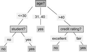
With the model now ready, a new record is submitted to this model, and the model will look at the input variables and traverse the nodes of the tree in Figure 1.7 to see where the new record falls. So, if the age on the new record is 23, it will be sent to the left node below age to check the student status. If that is yes, then the prediction result will be yes. So the input data and the model work to predict the outcome when it is not known. This is shown in Figure 1.8.

The basic concept of these examples of clustering and decision trees has been derived from the data mining course materials by Jiawei Han of the University of Illinois at Urbana-Champaign (Han, 2011) and Sajjad Haider of the Institute of Business Administration, Karachi, and the University of Technology, Sydney (Haider, 2012).
Text Mining
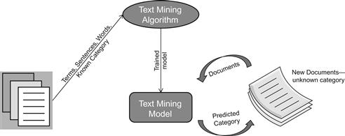
Text mining is used to predict lines, sentences, paragraphs, or even documents to belong to a set of categories. Since it predicts the category (of text) based on learning of similar patterns from prior texts, it qualifies to be a predictive analytics method. Although text mining does not use any of the classification or regression techniques, it is conceptually identical to prediction when it is being used to learn categories of text from a precategorized collection of texts, and then use the trained model to predict new incoming documents, news items, paragraphs, etc. Interestingly, another form of text mining can use clustering to see which news items, tweets, customer complaints, and documents are “similar,” so text mining can fall both under descriptive or predictive analytics based on how it is used. To keep things simple, let’s take the example of a news story prediction text mining solution. Thousands of documents containing past news stories are assigned categories like business, politics, sports, entertainment, etc. to prepare the training set.
The text mining algorithm uses this training set and learns the words, terms, combination of words, and entire sentences and paragraphs that result in labeling the text to be a certain category. Then, when new text is submitted, it tries to look for the same patterns of terms, words, etc. to see which known category the new text closely resembles and assigns that category to the text. Figure 1.9 illustrates a simple text mining example.
Decision Optimization
Decision optimization is a branch of mathematics that deals with maximizing the output from a large number of input variables that exert their relative influence on the output. It is widely used in economics, game theory, and operations research with some application in mechanics and engineering. Let’s use an example to understand where decision optimization fits into an organization’s activities. Suppose ABC Trucking is a transportation and logistics company that owns 20 trucks. Trucks make the most money for the company when they are full and on the road. ABC Trucking has the following entities or groups of variables:
■ Truck (truck type, age, towing capacity, engine size, tonnage, fuel capacity, hazardous material certification, etc.)
■ Driver (salary, overtime pay grade, route specialty, license classification, hazardous material training, etc.)
■ Shipment order (type, size, weight, invoice amount, delivery schedule, destination, packing restrictions, etc.)
The trucking company wants to maximize the use of its trucks and staff for the highest possible profits, but they have to deal with client schedules, hazardous materials requirements, availability of qualified drivers, cost of delivery, availability of appropriate trucks and trailers, etc. They wouldn’t want to travel with the truck half empty, they wouldn’t want to pay overtime to the driver, they wouldn’t want the truck to come back empty, and they wouldn’t want to miss the delivery schedule and face penalties or dissatisfied customers.
The complexity of this problem increases with the incoming shipment orders not having a well-defined or fixed pattern like seasonal volumes. This is the problem that decision optimization models try to solve. It provides the best possible drivers, combination of orders, and routing of the trucks to ensure trucks are not traveling empty, drivers are not overworked, and customers are satisfied. The analysis involves a correlation between variables and maximizing the output. The output in this case would be a routing and shipping schedule that has to be followed during a given time period. This is the scenario where analytics is answering the question of what should be done. Decision optimization always deals with a wide variety of alternates (Murty, 2003) to pick from and tries to find the best possible solution with the given targets. Decision optimization uses linear and nonlinear programming to solve these problems and is usually not considered part of machine learning or data mining. Rather it falls under the field of operations research.
Throughout this book, prediction examples will be used to explain the analytics solution implementation methodology and value for solving business problems, but it applies equally to other techniques like forecasting and optimization.
Conclusion of Definition
The most important part of these definitions is to understand the use of the technique so the correct technique is applied to the correct problem. Chapter 3 is fully dedicated to showing a wide variety of problems and applications of appropriate analytics techniques. There are additional analytics techniques such as:
These techniques all fall under data mining techniques, but are left out deliberately for future discussion as their adoption requires a certain degree of analytics maturity within the organization. Also, the implementation methodology presented here requires some boundaries around analytics techniques and methods, otherwise it would not be possible to show how consistent processes, infrastructure, and manpower can be developed to build and deliver analytics solutions repeatedly. This book is intended to take readers through the introductory stages of adopting analytics as a business and technology lifestyle and become evangelists of this paradigm. Advanced techniques, advanced software, and more complex business problems and solutions will follow naturally.