
Getting Familiar with Audio Signals
Abstract
The purpose of this chapter is to provide basic knowledge and techniques related to the creation, representation, playback, recording and storing of audio signals using MATLAB. In addition, short-term audio analysis is introduced here.
Keywords
MATLAB
Playback
Recording
Audio signals
Short-term
WAVE files
MP3
Nyquist
Sample rate
Short-term processing
The goal of this chapter is to provide the basic knowledge and techniques that are essential to create, playback, load, and store the audio signals that will be analyzed. Therefore, we focus on certain practical skills that you will need to develop in order to prepare the audio signals on which the audio analysis methods of later chapters will be applied. Although we have intentionally avoided overwhelming the reader with theory at this stage, we provide certain pointers to the most important theoretical issues that will be encountered. Our vehicle of presentation will be the MATLAB programming environment and even though the source code may not be directly reusable in other software development platforms, the presented techniques are commonplace and highlight certain key issues that emerge when it comes to working with audio signals, e.g. the difficulties in manipulating voluminous data.
2.1 Sampling
Before we begin, it is worth noting that, in principle, digital audio signals can be easily represented in the MATLAB programming environment by means of vectors of real numbers, as is also the case with any discrete-time signal. The term discrete time refers to the fact that although in nature time runs on a continuum, in the digital world we can only manipulate samples of the real-world signal that have been drawn on discrete-time instances. This process is known as sampling and it is the first stage in the creation of a digital signal from its real-world counterpart. The second stage is the quantization of the samples, but for the moment we will ignore it.
To give an example, the first sample may have been taken at time 0 (the time when measurement commenced), the second sample at 0.001 s, the third one at 0.002 s, and so on. In this case, the time instances are equidistant and if we compute the difference between any two consecutive time instances the result is ![]() , where
, where ![]() is known as the sampling period. In other words, one sample is drawn every
is known as the sampling period. In other words, one sample is drawn every ![]() . The inverse of
. The inverse of ![]() is the celebrated sampling frequency, i.e.
is the celebrated sampling frequency, i.e. ![]() . The sampling frequency is measured in Hz and in this example it is equal to
. The sampling frequency is measured in Hz and in this example it is equal to ![]() i.e. 1000 samples of the real-world signal are taken every second.
i.e. 1000 samples of the real-world signal are taken every second.
A major issue in the context of sampling is how high the sampling frequency should be (or equivalently, how short the sampling period has to be). It turns out that in order to successfully sample a continuous-time signal, the sampling frequency has to be set equal to at least twice the signal’s maximum frequency [1]. This lower bound of the sampling frequency is known as the Nyquist rate and it ensures that an undesirable phenomenon known as aliasing is avoided. More details on aliasing will be given later in this book but for the moment it suffices to say aliasing introduces distortion, i.e. it reduces the resulting audio quality.
2.1.1 A Synthetic Sound
In order to demonstrate the sampling process, we could simply start with a recording device and set its recording parameters to appropriate values so as to achieve a good quality recorded signal. However, we embark on an alternative route; we start with an example that creates a synthetic sound. In other words, we are making a first attempt to simulate the sampling stage of the recording procedure by employing our basic sampling knowledge. More specifically, in the following script, three sinusoidal signals (tones) of different frequencies are synthetically generated and their sum is computed and plotted. The resulting signal is, therefore, a sum of tones and the tone of maximum frequency (900 Hz) determines the Nyquist rate. Therefore, in this case, a sampling frequency of at least 1800 Hz is required. The comments on each line explain the respective command(s). This is a style of presentation that we have preserved throughout this book.
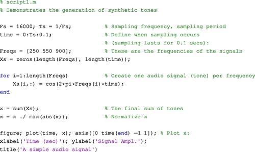
In order to understand how the script works, consider a simple tone (sinusoidal signal) in continuous time, with frequency 250 Hz, i.e. ![]() , where
, where ![]() is the amplitude of the tone (phase information has been ignored for the sake of simplicity). In our case,
is the amplitude of the tone (phase information has been ignored for the sake of simplicity). In our case, ![]() for each tone, meaning that each tone’s maxima and minima occur at +1 and −1, respectively. If
for each tone, meaning that each tone’s maxima and minima occur at +1 and −1, respectively. If ![]() is the sampling period then the samples are taken at multiples of
is the sampling period then the samples are taken at multiples of ![]() , where
, where ![]() is a positive integer and
is a positive integer and ![]() . In other words, our example first needs to implement the equation
. In other words, our example first needs to implement the equation ![]() for each tone and then sum the resulting signals. Note that the final audio signal is normalized by dividing it with its maximum value and as a result, the values in vector
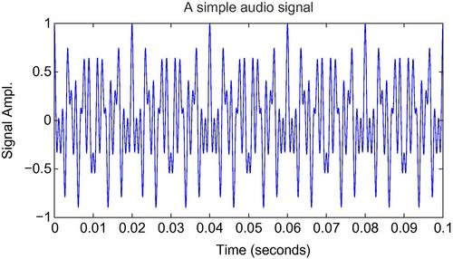
for each tone and then sum the resulting signals. Note that the final audio signal is normalized by dividing it with its maximum value and as a result, the values in vector ![]() lie in the range [−1,1]. Figure 2.1 presents the audio signal that is generated by the above script.
lie in the range [−1,1]. Figure 2.1 presents the audio signal that is generated by the above script.
2.2 Playback
A useful MATLAB command, which sends a vector (stream) of samples, x, to the sound card device for playback purposes is the sound(x,fs,nbits) command, where fs is the sampling frequency based on which x will be reproduced and nbits is the number of bits that are used to represent each sample (this number is also known as the sample’s depth and is determined during the quantization of samples). If the sampling frequency is not provided then a default value is assumed by MATLAB (around 8 KHz). Similarly, depending on the operating environment, the default bit representation may utilize 8 or 16 bits. In order to avoid distortion during the playback operation, the values in x have to be in the range [−1,1]. If you want to listen to the signal that was generated by the example in Section 2.1.1, type:
![]()
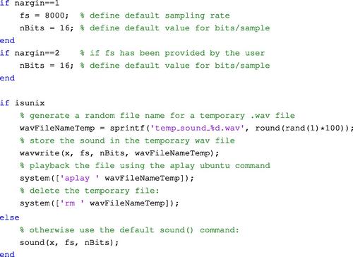
It is important to note that when using MATLAB with operating systems other than the MS Windows environment, certain sound playback issues may be encountered. For example, in the Ubuntu OS, the sound() command may lead to an error due to sound card compatibility issues. In order to circumvent such situations, we can resort to an alternative way to play a sound: we first store it in a temporary audio (WAVE) file and then we ‘play’ the file using an appropriate system utility. For example, in the Ubuntu OS, this functionality can be achieved by the aplay command-line utility, which automatically determines the sampling rate, number of bits per sample, and other properties of the sound-file format and then plays the respective sound. In this line of thinking, the following function can be used to reproduce a sound both in the MS Windows and Ubuntu operating systems:

2.3 Mono and Stereo Audio Signals
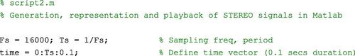
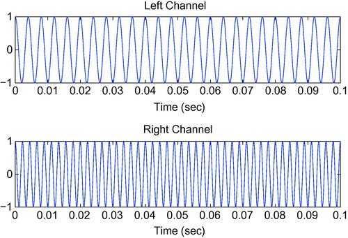
In MATLAB, a column vector represents a single-channel (monophonic—MONO) audio signal. Similarly, a matrix with two columns refers to a two-channel signal (stereophonic—STEREO), where the first column represents the left channel and the second column represents the right channel. The following code creates a STEREO signal. The left channel contains a 250 Hz tone (cosine signal) and the right channel a 450 Hz tone. Figure 2.2 provides a separate plot of each channel over time.

2.4 Reading and Writing Audio Files
2.4.1 WAVE Files
A common file format for uncompressed audio is the WAVE format which is built on pulse-code modulation (PCM) technique for the quantization of samples. The associated files are expected to have a ‘.wav’ extension. In MATLAB, the audio content of such files can be easily loaded into the workspace using the wavread() function (type help wavread for a detailed description of this function). The most important input argument of this function is a string which specifies the name of the WAVE file to be read:
![]()
Wavread() returns the audio signal, x; the sampling frequency, Fs, with which the signal was recorded (or synthetically generated); and the number of bits per sample, nBits. If the file contains a MONO audio signal, then x is a column vector, whereas, if the file contains a STEREO sound then x is a matrix of two columns, one column per channel. Wavread() can also be used to read excerpts (segments) of the audio content. The following call to wavread() loads into the workspace just the first N samples of the file:
![]()
It is also possible to read samples N1 through N2 from each channel by using the following syntax:
![]()
It is also possible to simply retrieve the length of the audio stream without actually reading the signal samples. This is feasible due to the structure of WAVE files. This structure has been standardized in the respective format specification and is reflected on the “header” of the file. The header is a chunk of data that reside in the beginning of the file and give various details including sampling frequency, depth of samples, number of channels, order with which the samples are stored, and so on. The following call to wavread() will therefore only retrieve header information from file ‘test.wav.’
![]()
The first output variable, SIZE, contains two elements: the number of samples and the number of channels. As a result, to compute the time duration of the audio signal (in seconds), type
![]()
In order to store an audio signal, x, into a WAVE file, the wavwrite() function can be used (type help wavwrite for a detailed description of input and output arguments). In summary, the input arguments for this function are: the signal, x (column vector or two-column matrix); the sampling frequency, Fs; the number of bits per sample, and the name of the file to create.
![]()
Note that the above function call results in a destructive operation, in the sense that, if the file already exists, then its content will be overwritten. For the reader who is interested in the technicalities of wavwrite(), we provide a few more details: if x is a vector of floating-point numbers, then the number of bits per sample can be 8, 16, 24, or 32 and each element of x should preferably lie in the range [−1,1]. If a value falls outside the previous range, an operation known as ‘clipping’ will be performed (one of the exercises in this chapter involves the clipping technique). The elements of x may also be of other data types, e.g. of the int16 data type (16-bit integers covering the range of integers ![]() ). In such cases, the reader is encouraged to consult the help utility of the function in order to determine which values are allowable for the number of bits per sample.
). In such cases, the reader is encouraged to consult the help utility of the function in order to determine which values are allowable for the number of bits per sample.
2.4.2 Manipulating Other Audio Formats
MATLAB supports some other standard audio formats further to the WAVE format. For example, function auread() can be used to load audio stored in ‘.au’ files. The Au file format [2] provides a simple interface for audio storage and its philosophy bears certain similarities with the WAVE format specification. The Au file format has a simple header and uses simple encoding schemes for the audio data, including 8-bit ![]() -law and 8-,16-,24-,32-bit linear PCM. As with the syntax of wavread(), auread() also returns the signal samples in an array and the sampling frequency and bits per sample in separate output variables.
-law and 8-,16-,24-,32-bit linear PCM. As with the syntax of wavread(), auread() also returns the signal samples in an array and the sampling frequency and bits per sample in separate output variables.
Another very popular format, for which it is useful to have a MATLAB encoder and decoder, is the MP3 format, which is based on the principles of perceptual coding [3,4]. MP3 is a lossy format, in the sense that the decoded signal is not identical to the original one. Until recently, MATLAB did not support I/O for MP3 files and developers had to rely on 3d-party software. Lately, the audioread function was added to the MATLAB environment, making it possible to manipulate MP3 audio data from the workspace. Note that audioread() is not restricted to MP3 files and serves as a root function which is aimed at addressing various audio data formats. Its syntax is similar to the syntax of wavread() and auread().
An alternative way to read audio data of (almost) every popular format, including the aforementioned formats, is by using the ffmpeg command-line tool of the FFmpeg multimedia framework (1). At the time of writing, the FFmpeg suite of tools was a GNU-LGPL and GNU-GPL licensed cross-platform framework. The goal of the FFmpeg project is to allow users to engage with various multimedia processing operations, including the loading and storage of audio data and the conversion among audio data types. The FFmpeg framework uses its own codecs (implementations of coding-decoding schemes) for data processing and its functionality is available to program developers (e.g. C/C++ program developers) by means of an appropriate application programming interface (API). In the rest of this section, we present on a by-example basis, the functionality of the FFmpeg tool of the FFmpeg project with respect to audio processing; and we show how this functionality can be made available to MATLAB routines (the toolkit of the FFmpeg project includes the ffserver, ffplay, and ffprobe tools).
For the moment, let us ignore MATLAB and assume that we want to transform an MP3 file, say ‘file.mp3’ to the WAVE file ‘output.wav.’ This type of processing is also known as transcoding because we transform a data stream from one coding scheme to another. To this end, start a terminal window and type:
ffmpeg -i file.mp3 output.wav
It is also possible to transcode selected parts of the audio stream. For example, if you type:
ffmpeg -i file.mp3 -t 5 output.wav
then the first 5 s of the audio signal in file.mp3 are transcoded and stored to file output.wav.
Another useful parameter that can be passed to the FFmpeg tool as a command-line argument is the -ar <value> flag, which sets the sampling rate for the output file. In a similar manner, flag -ac sets the number of output channels. Therefore, the command
ffmpeg -i file.mp3 -ar 16000 -ac 1 output.wav
extracts the audio signal from file.mp3, resamples it at 16 KHz, converts it to a single-channel representation, and stores it to file output.wav.
In the library of MATLAB functions that we provide with this book, you will find the function mp3toWav(), which simply uses MATLAB function system() to call the FFmpeg tool in order to transcode an MP3 file to the WAVE format. In addition, function mp3toWavDIR() transcodes all MP3 files in a folder to their WAVE counterparts. For each successful audio stream conversion, a new file is created, preserving the original filename and modifying the extension to address the new file format.
Finally, note that you will encounter several examples of MATLAB code on the Internet where the FFmpeg toolkit is used to handle various types of multimedia content. The MATLAB Central website for File Exchange can be a good source for the interested reader. An example is the mmread() function (authored by Micah Richert, available via the Mathworks File Exchange website,2) which is based on the joint use of FFmpeg and AVbin.
2.5 Reading Audio Files in Blocks
As explained in Section 2.5, if an audio file is very large, loading all its contents into memory may be impractical. Consider, for example, a .wav file in which a 3-minute music track has been stored. The sampling frequency is assumed to be 44100 Hz (CD quality recording) and two channels have been used (STEREO mode). If we consider that MATLAB uses by default double-precision floating-point arithmetic for its variables (i.e. each variable is by default 8 bytes long), then the total number of bytes needed to load this music track into memory is: ![]() . Usually, there is no need to keep the whole signal in memory all the time, because, in most applications, the audio signals are processed on a short-term basis. (See Section 2.7 for more details on short-term processing.)
. Usually, there is no need to keep the whole signal in memory all the time, because, in most applications, the audio signals are processed on a short-term basis. (See Section 2.7 for more details on short-term processing.)
The goal of the next example is to demonstrate block-based audio processing, a simple technique to overcome the need for loading and keeping all the contents of the audio file into memory. The corresponding function is readWavFile(). You will need to execute the following steps:
• Determine the total number of audio samples and the sampling frequency, using the ‘size’ option in the call to the wavread() function:

• Use a while loop for reading one block of the audio signal each time. The limits of each block (indices of leftmost and rightmost sample) need to be provided in the call to the wavread() function:
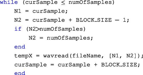
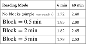
Concerning response times, the block-reading mode introduces a small delay due to the repeated calls to the wavread() function (one call per block). However, this is not a crucial issue as it can be also seen in Table 2.1, where the execution times are presented for different files on a standard laptop. Note that if your application demands for efficient IO handling, then you probably need to resort to an alternative implementation of the wavread() function. For example, you can re-engineer the wavread() function so that the audio file is left open throughout the whole reading operation, thus reducing certain IO overheads.
Execution Times for Different Loading Techniques
| Reading Mode | 6 min | 48 min |
| No blocks (simple wavread()) | 1.72 | 2.40 |
| 1.83 | 2.80 | |
| 1.82 | 2.65 | |
| 1.78 | 2.53 |
2.6 Recording Audio Data
2.6.1 Audio Recording Using the Data Acquisition Toolbox
In order to read data from a sound card, you can use the Data Acquisition Toolbox of MATLAB. In addition to sound recording, this toolbox also provides functionality for controlling various types of data acquisition hardware. In order to use the Data Acquisition Toolbox for audio recording, you need to follow the steps given in Table 2.2.
Sound Recording Using the Data Acquisition Toolbox
| Step | Description |
| 1 | Create a device object |
| 2 | Add channels |
| 3 | Configure recording properties |
| 4 | Initialize recording |
| 5 | Trigger recording |
| 6 | Acquire data |
| 7 | Terminate process |
It is worth noting that if steps 4–6 are nested inside a loop, then each data block can be processed separately, right after it has been acquired. This is useful when it is desirable to perform online audio processing operations.
Let us now review the basic steps of the recording procedure in more detail. The first two steps create a sound card object and add an audio channel to that object. The audio object serves as an operation handler, i.e. the object is the gateway via which the recording procedure is actually implemented:
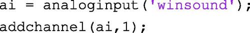
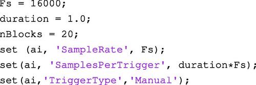
The winsound string, which is given as input to the analoginput function defines that the sound card object is created using an MS Windows driver. Our next concern is to set values for a number of recording parameters, namely, the sampling frequency (SampleRate), the length of the recording block (SamplesPerTrigger), and the triggering mode (TriggerType). The last parameter defines that the recording times are manually controlled. As can be seen in the following code, for each recording parameter we need to set the value of the respective object attribute:
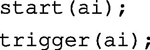
Then, inside a loop (i.e. for each block), we initialize (start) and begin (trigger) the recording process:
Inside the loop, we use a variable (x) to store each block of acquired data:
![]()
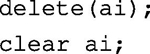
After the data acquisition loop has ended, we clear the previously created acquisition handler:
The reader may refer to script3.m for the complete version of the above audio recording procedure. The functionality in script3.m can be summarized as follows:
• Twenty blocks of audio data are recorded in total. Each block is 1.0 s long.
• A buffer is used to store the complete audio recording. This is done mainly for educational purposes and it may not be necessary in many applications, for reasons that were previously stated.
• At each iteration, while the current block is being recorded, the intensity of the signal (in dB) is computed for the previous block and is plotted using a simple bar plot.
• In the end, the contents of the audio buffer are stored in a WAVE file.
2.6.2 Audio Recording Using the Audio Recorder Function
The recording procedure of Section 2.6.1 is just one technique for sound recording with MATLAB. An alternative approach is to use the audiorecorder function. Note that this methodology does not support disk buffering. Instead, it stores the audio samples in the computer memory. It is, therefore, not the best solution when the expected recording duration is very long. If, however, the function is used in a block-processing context, as in the following example, the memory usage issues can be circumvented because intermediate audio data blocks can be stored on a disk.
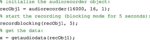
In order to use the audiorecorder() function, we first need to set the parameters of the recording procedure (i.e. the sampling frequency, the number of bits per sample, and the number of channels). We then use the audiorecorder constructor to create a recording object (recObj1):

After the recording object has been created, the actual recording process is started:
![]()
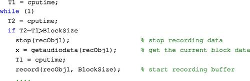
BlockSize is the duration of each block to be recorded and record is a non-blocking function, i.e. a function that returns immediately, making it suitable for online (block-based) processing applications. In the context of block-processing procedures, a MATLAB timer can be adopted for synchronization purposes (e.g. using MATLAB’s cputime() function). In that case, a loop is used and at each iteration, we measure the elapsed time since the beginning of the recording of the current block. If the elapsed time exceeds the desired length (in seconds) of the recording block, then we: (a) stop the recording process, (b) get the audio data of the last block and store it in a variable, and (c) restart the recording process, along with the MATLAB timer:
The process is repeated until the desired number of blocks has been acquired. The script4 m-file provides a detailed demonstration of the audiorecorder() function in the context of the block-processing (online) mode of operation (the design of the rest of the script has been kept similar to the example of Section 2.6.1).
Note: Instead of using the record() function, we can alternatively use the recordblocking() function, which does not return control until recording completes. The second argument for that function is the duration of the data to be recorded. In this way, the resulting code becomes rather simple:
The script4 m-file is using ‘manually’ controlled synchronization. However, MATLAB provides yet another method for the online processing of recorded data, i.e. the mechanism of callback functions. More specifically, a property named TimerFcn of the audiorecorder object can be set to define the callback function that will be executed repeatedly during the recording procedure. To specify the periodicity of repetitions, it is necessary to set the TimerPeriod property of the audiorecorder object. For example:
![]()
In the above lines of code, someFunction is the name of the callback function to be executed every 0.5 s. An example of such a callback function is the audioRecorderTimerCallback() function that we provide in the software library of this book. That function is used by audioRecorderOnline, which simply initializes the audiorecorder object. In other words, audioRecorderTimerCallback() defines the processing steps which need to be applied on the recorded data at every iteration. In the provided example, we simply plot the signal samples at each recording stage. In order to execute this callback-based audio recording procedure, simply call the initialization function from the MATLAB workspace:
![]()
2.7 Short-term Audio Processing
In most applications, the audio signal is analyzed by means of a so-called short-term (or short-time) processing technique, according to which the audio signal is broken into possibly overlapping short-term windows (frames) and the analysis is carried out on a frame basis. The main reason why this windowing technique is usually adopted is that the audio signals are non-stationary by nature, i.e. their properties vary (usually rapidly) over time [5]. Let us ignore for the moment the mathematical formalism and try to understand, by means of a simplified example, what non-stationarity stands for. More specifically, consider an audio recording consisting of a short conversation (1 s long) between two individuals, that is followed by the shout of a third person (also 1 s long). Therefore, this audio recording consists of two main events: the conversation (normal intensity signal) and the shout (high-intensity signal). It is obvious that the signal changes abruptly from the state of the conversation to the state of the shout. From a very simplified perspective, this can be considered as a change of stationarity, i.e. the properties of the signal shift from one state to another. In such situations, it would not really make sense to compute, for example, the average intensity of the samples of the whole recording because the resulting value would be dominated by the more intense samples that were recorded during the shout of the third person. Instead, it would be more useful to break the recording into short segments and compute one value of (average) intensity per segment. This is also the main idea behind short-term processing. Of course, it has to be noted that in our example, the change of stationarity was observed at the more abstract level of audio events, whereas short-term processing usually works at the microcosm of the samples of the signals.
To continue, let ![]() , be an audio signal,
, be an audio signal, ![]() samples long. During short-term processing, we focus each time on a small part (frame) of the signal. In other words, we are following a windowing procedure: at each processing step, we multiply the audio signal with a shifted version of a finite duration window function,
samples long. During short-term processing, we focus each time on a small part (frame) of the signal. In other words, we are following a windowing procedure: at each processing step, we multiply the audio signal with a shifted version of a finite duration window function, ![]() , i.e. a discrete-time signal which is zero outside a finite duration interval. The resulting signal,
, i.e. a discrete-time signal which is zero outside a finite duration interval. The resulting signal, ![]() , at the
, at the ![]() processing step is given by the equation:
processing step is given by the equation:
where ![]() is the number of frames and
is the number of frames and ![]() is the shift lag, i.e. the number of samples by which the window is shifted in order to yield the
is the shift lag, i.e. the number of samples by which the window is shifted in order to yield the ![]() frame. Equation (2.1) implies that
frame. Equation (2.1) implies that ![]() is zero everywhere, except in the region of samples with indices
is zero everywhere, except in the region of samples with indices ![]() , where
, where ![]() is the length of the moving window (in samples). The value of
is the length of the moving window (in samples). The value of ![]() depends on the hop size (step),
depends on the hop size (step), ![]() , of the window. For example, if the window is shifted by 10 ms at each step and the sampling frequency,
, of the window. For example, if the window is shifted by 10 ms at each step and the sampling frequency, ![]() , is 16 kHz, then,
, is 16 kHz, then, ![]() samples,
samples, ![]() . Furthermore, if
. Furthermore, if ![]() samples, then the 5th frame (
samples, then the 5th frame (![]() ) starts at sample index
) starts at sample index ![]() and ends at sample index
and ends at sample index ![]() .
.
The above highlights the fact that the important parameters of the short-term processing technique are the length of the moving window, ![]() , its hop size (step),
, its hop size (step), ![]() , and its type (the function used to implement the window). Usually,
, and its type (the function used to implement the window). Usually, ![]() varies from 10 ms to 50 ms. On the other hand, the window step,
varies from 10 ms to 50 ms. On the other hand, the window step, ![]() , controls the degree of overlap between successive frames. If, for example, a
, controls the degree of overlap between successive frames. If, for example, a ![]() overlap is desired and the window length is 40 ms, then the window step has to be 10 ms. It can be easily derived that the total number,
overlap is desired and the window length is 40 ms, then the window step has to be 10 ms. It can be easily derived that the total number, ![]() , of short-term windows is equal to:
, of short-term windows is equal to:

where ![]() , and
, and ![]() were defined above and
were defined above and ![]() is the floor operator. Figure 2.3 presents an example of short-time processing where the length of the moving window is 200 samples and its hop size is 100 samples (
is the floor operator. Figure 2.3 presents an example of short-time processing where the length of the moving window is 200 samples and its hop size is 100 samples (![]() overlap between successive windows).
overlap between successive windows).

Figure 2.3 Short-term processing of an audio signal. Three consecutive frames are shown. Each frame is 200 samples long and a ![]() overlap exists between successive frames.
overlap exists between successive frames.
Concerning the window types that can be used, the simplest choice is the rectangular window (MATLAB rectwin() function), in which the signal is simply truncated outside the limits of the window and is left unaltered inside the window. Equivalently, each sample inside the region defined by the window is multiplied by 1, whereas all the other samples are multiplied by 0. This is also described in the following equation:
Further to the rectangular window, other choices (which are also supported by MATLAB) are the popular Hamming window, the Bartlett window, and the Hanning window, to name but a few. What differs between those window types is the function that determines the shape of the window, i.e. the attenuation near the edges of the window, the smoothness of the respective curve, and so on.
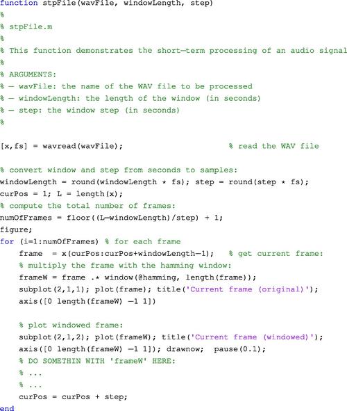
The stpFile() function demonstrates the short-term processing technique. The source code of this function has been kept simple for educational purposes and it is not optimal in any sense. If we go through this m-file, we can see that it first copies each frame in a temporary vector and it then multiplies the contents of the vector by the Hamming window. Of course, the Hamming window can be substituted by any valid window function. Finally, for each frame, the original and the windowed versions are plotted. From a technical perspective, if the audio file is too large then we may need to read it in blocks (as was shown in Section 2.5). In such cases, the short-term processing technique has to be applied separately on each block.
2.8 Exercises
1. (D1) Write a MATLAB function that reads the header of a WAVE file (the path to the file is the first argument of the function) and checks if the stored audio signal is in STEREO mode. If this is the case, then the signal is loaded, it is converted to MONO mode, and it is stored to a new WAVE file (second input argument). During this procedure the sampling frequency is left unaltered.
2. (D2) The stpFile() function described in Section 2.5, which can be found in the repository that accompanies the book, demonstrates a short-term processing technique that plots the short-term frames of a given signal. In this exercise, you are asked to modify the plotting procedure, so that the horizontal axis presents the time in seconds instead of showing sample indices.
3. (D3) Write a MATLAB function that:
(a) Uses the audiorecorder functionality (Section 2.6.2) to record 1 s of audio data. The process is repeated twice, i.e. two 1-sec audio segments are sequentially recorded.
(b) Creates a STEREO signal by placing each recorded segment in a separate channel.
(c) Plays the STEREO signal.
4. (D3) If the audiorecorder functionality is nested inside a loop (Section 2.6.2), it can be used to record large amounts of data provided that the data are saved on a hard disk, progressively. In that way, there is no need to store the entire signal into memory. Write a MATLAB program that:
(a) Uses the audiorecorder functionality to record a number of audio segments, where each segment is 10 s long. This can be achieved, either by adopting the loop-based procedure of script4 or by using the callback-based approach (Section 2.6.2).
(b) Stores each segment in a separate WAVE file (for example, segment 1 is stored in file output0001.wav, segment 2 in output0002.wav, and so on).
Note that, since only 10 s of audio are stored in memory at each recording stage (and the rest on hard disk), the above procedure can be used to record arbitrarily long audio streams.
5. (D4) In this exercise you are asked to create a MATLAB function that:
(a) Repeats the first step of the previous exercise.
(b) For the current segment, the intensity of the signal is computed (in dB) as in script4, i.e. using the command 10*log10(mean(x.ˆ2)), where x is the vector of the samples of the segment.
(c) If the intensity level of a segment is higher than a predefined threshold (e.g. −20 dB) then the respective segment is stored in a WAVE file, otherwise the process continues with the next segment. In order to name each WAVE file that is automatically created, you may either use a timestamp that is derived from the elapsed execution time or a simple counter that counts the number of segments that survived the threshold. You may find it useful to employ MATLAB’s cputime and clock functions.
Similar to the previous exercise, the computer’s memory does not need to store the whole signal. However, unlike the previous exercise, not every segment is stored in a WAVE file; only segments with sufficient energy are preserved. This type of functionality can be used to monitor long periods of audio activity while storing only selected audio segments on the disk. Consider for example, an audio surveillance application, where the monitoring operation should never cease. If the solution to this exercise was adopted, there would be no need to store every audio sample on the disk, only those parts of the audio stream that correspond to high-intensity signals.
6. (D2) Section 2.4.2 described how to transcode MP3 files to the WAVE format by calling the external FFmpeg tool. The object of this exercise is to write a MATLAB function that achieves the following goals:
(a) Receives as its first input argument the full path to an MP3 file and checks if the file exists.
(b) If it exists, the FFmpeg tool is called to convert the MP3 file to a temporary WAVE file.
(c) It plots and plays the signal in the temporary file.
(d) It deletes the temporary file.
7. (D5) MATLAB provides the Graphical User Interface Development Environment (GUIDE) for the creation of Graphical User Interfaces (GUIs). In this exercise, you are asked to:
(a) Use GUIDE to create a simple user interface composed of: (a) a LOAD button, (b) a PLAY button, (c) a SAVE button, (d) two plotting areas, and (e) two sliders (one slider below each plotting area).
(b) When the LOAD button is pressed, a file selection dialog appears that lets the user select a WAVE file. To this end, use the uigetfile() function. If the selected WAVE file is in STEREO mode, then each channel is plotted separately in the respective plotting area. If not, the same signal is plotted on both areas. Furthermore, if the signal is in MONO mode, a STEREO signal is synthesized by using the same signal in both channels.
(c) The two sliders are used to amplify the respective channels. The amplification is achieved by simple multiplication of each channel with the factor defined by the slider. Each slider produces values in the range [0,5], with values ![]() attenuating the signal and values
attenuating the signal and values ![]() amplifying it.
amplifying it.
(d) When the PLAY button is pressed, the signal is played. Furthermore, if the SAVE button is pressed then the signal is stored in a predefined WAVE file.
8. (D5) One way of loading video files in MATLAB is by creating objects of the VideoReader class. In this exercise you are asked to develop a MATLAB program that:
(a) Takes as input the path to a video file (AVI format), calls the FFmpeg tool to extract the audio signal from the video file and stores the signal into a WAVE file.
(b) Applies short-term processing (Section 2.7) on the audio signal and computes the average absolute value of the samples in each frame. The length of the moving window is equal to 100 ms with zero overlap between successive windows. The result of this stage is a sequence of values.
(c) Detects the maximum value of the previous sequence and assumes that the time instant, ![]() , at which this value occurs coincides with the time equivalent of the center of the respective frame.
, at which this value occurs coincides with the time equivalent of the center of the respective frame.
(d) Retrieves the video frame that corresponds to ![]() and uses the imshow()) function to display it.3
and uses the imshow()) function to display it.3
9. (D4) Center clipping is a useful technique according to which a signal sample survives if its absolute value exceeds a predefined threshold. Equation (2.3) defines the clipping operation when a single threshold, ![]() , is used.
, is used.
where ![]() and
and ![]() are the clipped and original signal, respectively. In this exercise, you are asked to develop a function that receives as input a monophonic audio signal and a clipping threshold and plots the clipped signal on a short-term processing basis. You may find it useful to reuse parts of the source code of function stpFile(). The length and step of the moving window are user-defined parameters.
are the clipped and original signal, respectively. In this exercise, you are asked to develop a function that receives as input a monophonic audio signal and a clipping threshold and plots the clipped signal on a short-term processing basis. You may find it useful to reuse parts of the source code of function stpFile(). The length and step of the moving window are user-defined parameters.
10. (D5) The object of this exercise is to develop a MATLAB program that shuffles an audio signal as follows:
• Starts with a WAVE file and reads its contents in block-mode. The block length, ![]() , is a user parameter.
, is a user parameter.
• Stores each block as the row of a matrix, say ![]() . Employs zero padding for the last block, if its length is shorter than
. Employs zero padding for the last block, if its length is shorter than ![]() .
.
• After all blocks have been read, shuffles the rows of matrix ![]() . To this end, function randperm can prove to be useful.
. To this end, function randperm can prove to be useful.
• Creates a new WAVE file by storing each row of ![]() , one after the other, in this new file.
, one after the other, in this new file.
• Listens to the result.
Depending on the original file, shuffling can create an audio effect that can be used as a tapestry of sounds in the background of a recording. This is a well-known technique in music recording studios. Finally, create a stereo recording by placing the shuffled audio signal in the left channel and a signal of your choice in the right channel. Save the result and listen to it.
2 http://www.mathworks.com/matlabcentral/fileexchange/8028-mmread![]() .
.
3 The VideoReader class may not be available for older versions of MATLAB. In which case, you can alternatively use the mmread() function, which is available in the Mathworks File Exchange website (http://www.mathworks.com/matlabcentral/fileexchange/8028-mmread![]() ).
).