
Signal Transforms and Filtering Essentials
Abstract
This chapter presents methods towards the representation of audio signals in the frequency domain. Special emphasis has been placed on the description of the Discrete Fourier Transform because a lot of material in later chapters of this book assumes that the reader is familiar with this particular transform. Furthermore, the chapter aims at presenting the fundamentals of digital filters in MATLAB, so that, in the end of this chapter, the reader will be able to create and experiment with basic filter types and understand how they can affect the performance of various audio analysis stages.
Keywords
Discrete Fourier Transform
DFT
Fast Fourier Transform
FFT
Short-Time Fourier Transform
STFT
Aliasing
Discrete Cosine Transform
DCT
Discrete Time Wavelet Transform
DTWT
FIR filter
IIR filters
dB
Pre-emphasis
fdatool
Noise
The goal of this chapter is to provide a gentle introduction to selected signal transforms, which generate representations that are useful in various audio-related tasks, including feature extraction, compression, and multiresolution analysis, to name but a few. We have placed special emphasis on the description of the Discrete Fourier Transform because a lot of material in later chapters of this book assumes that the reader is familiar with this particular transform. We also present the fundamentals of digital filters, so that, by the end of the chapter, the reader will be able to create and experiment with basic filter types and understand how they can affect the performance of various audio analysis stages.
3.1 The Discrete Fourier Transform
The Discrete Fourier Transform (DFT) is of paramount importance in all areas of digital signal processing. It is used to derive a frequency-domain (spectral) representation of the signal. As will be made clear in the next chapter on feature extraction, the majority of the important features used to analyze audio content are defined in the frequency domain. It is, therefore, important to gain a firm understanding of the DFT. To this end, we will focus on presenting the transform from an implementation perspective and our discussion will evolve around the interpretation of the output of the DFT and how it reflects the properties of the audio signal. Before we proceed, note that an efficient algorithm for the computation of the DFT coefficients is the Fast Fourier Transform (FFT), which exploits the computational redundancy in the equations that define the DFT and its inverse transform.
Given a discrete-time signal, ![]() ,
, ![]() samples long, its DFT is defined as:
samples long, its DFT is defined as:
where ![]() . It can be observed that the output of the transform is a sequence of
. It can be observed that the output of the transform is a sequence of ![]() coefficients, the
coefficients, the ![]() , which, in general, are complex numbers. The DFT coefficients constitute the frequency-domain representation of the signal, which is further explained later in this chapter.
, which, in general, are complex numbers. The DFT coefficients constitute the frequency-domain representation of the signal, which is further explained later in this chapter.
The inverse DFT (IDFT) takes as input the DFT coefficients and returns the original signal:

Equation (3.2) provides an exact reconstruction of the original signal. As a result, the time-domain signal, ![]() and the complex signal,
and the complex signal, ![]() can be treated as equivalent representations. If we rewrite Eq. (3.2) in the form
can be treated as equivalent representations. If we rewrite Eq. (3.2) in the form

where ![]() , then it can be seen that the original signal,
, then it can be seen that the original signal, ![]() , can be written as a weighted average of a family of fundamental signals (basis functions), where each signal,
, can be written as a weighted average of a family of fundamental signals (basis functions), where each signal, ![]() , is a complex exponential and its weight is equal to the
, is a complex exponential and its weight is equal to the ![]() th DFT coefficient.
th DFT coefficient.
A useful interpretation of the DFT coefficients, in which we are particularly interested for practical reasons, is that, if ![]() is the sampling frequency that was used to obtain
is the sampling frequency that was used to obtain ![]() , then the
, then the ![]() th exponential corresponds to the analog frequency
th exponential corresponds to the analog frequency ![]() (the discrete-time equivalent of which is
(the discrete-time equivalent of which is ![]() ). For a given sampling frequency, larger values of
). For a given sampling frequency, larger values of ![]() (i.e. longer signals) result in a more dense sampling of the frequency axis, because
(i.e. longer signals) result in a more dense sampling of the frequency axis, because ![]() becomes smaller. Therefore, a larger value of
becomes smaller. Therefore, a larger value of ![]() is expected to produce a finer representation of the signal in the frequency domain, i.e. a better frequency resolution. However, there is a subtle issue here, which we will demonstrate later on by means of certain examples: the whole discussion on increasing frequency resolution is valid, as long as the signal remains stationary, i.e. as long as its properties do not change over time. For example, a sum of sinusoids of very long duration is a stationary signal, which can be easily studied with high-frequency resolution. On the other hand, if a signal changes from a sum of two sinusoids to a sum of three sinusoids, it is no longer stationary. It can only be considered stationary on a local basis. In such situations,
is expected to produce a finer representation of the signal in the frequency domain, i.e. a better frequency resolution. However, there is a subtle issue here, which we will demonstrate later on by means of certain examples: the whole discussion on increasing frequency resolution is valid, as long as the signal remains stationary, i.e. as long as its properties do not change over time. For example, a sum of sinusoids of very long duration is a stationary signal, which can be easily studied with high-frequency resolution. On the other hand, if a signal changes from a sum of two sinusoids to a sum of three sinusoids, it is no longer stationary. It can only be considered stationary on a local basis. In such situations, ![]() cannot increase arbitrarily. As a consequence, we cannot always achieve the desirable frequency resolution, because
cannot increase arbitrarily. As a consequence, we cannot always achieve the desirable frequency resolution, because ![]() is constrained by the stationarity changes in the signal. In other words, we need to resort to a trade-off between frequency and time resolution.
is constrained by the stationarity changes in the signal. In other words, we need to resort to a trade-off between frequency and time resolution.
Another discussion in which we are particularly interested involves the magnitude of the ![]() th DFT coefficient,
th DFT coefficient, ![]() , which can be treated as a measure of the intensity with which the respective frequency participates in the signal
, which can be treated as a measure of the intensity with which the respective frequency participates in the signal ![]() . This leads us to the aforementioned spectral interpretation of the DFT. Note that the phase of the DFT coefficients can also play a useful role in various applications and its role should not be underestimated. However, the majority of feature extraction methods are heavily based on the magnitude of the DFT coefficients.
. This leads us to the aforementioned spectral interpretation of the DFT. Note that the phase of the DFT coefficients can also play a useful role in various applications and its role should not be underestimated. However, the majority of feature extraction methods are heavily based on the magnitude of the DFT coefficients.
MATLAB has adopted the FFTW open-source library [6], http://www.fftw.org![]() , for the implementation of the DFT. The respective built-in function is fft(). To compute the DFT of a one-dimensional signal, which is stored in the MATLAB vector x, type
, for the implementation of the DFT. The respective built-in function is fft(). To compute the DFT of a one-dimensional signal, which is stored in the MATLAB vector x, type
![]()
By the definition of the DFT, the length of vector ![]() is equal to the length of the input signal. An engineering trick that is often used in association with the computation of the DFT is the zero-padding technique. The goal of zero padding is to achieve increased frequency resolution to the expense of adding a number of zeros in the end of the input signal. To enable zero padding, call the fft() function as follows:
is equal to the length of the input signal. An engineering trick that is often used in association with the computation of the DFT is the zero-padding technique. The goal of zero padding is to achieve increased frequency resolution to the expense of adding a number of zeros in the end of the input signal. To enable zero padding, call the fft() function as follows:
![]()
where ![]() is the desired number of DFT coefficients, after zero padding has taken place. If the input signal is longer than
is the desired number of DFT coefficients, after zero padding has taken place. If the input signal is longer than ![]() samples then X is truncated.
samples then X is truncated.
The magnitude of the DFT coefficients can be easily computed by means of the abs() MATLAB function. As an example, type:

The vector of the resulting DFT coefficients is
![]()
Consequently, the output of the abs() function is
![]()
If we take a closer look at the DFT coefficients and their magnitude, we can verify a well-known property that is derived from the theory of the DFT: for a real-valued signal, the DFT coefficients appear in conjugate pairs, i.e. ![]() . This implies that the magnitude of the spectrum is symmetric. In the above example,
. This implies that the magnitude of the spectrum is symmetric. In the above example, ![]() and:
and: ![]() , etc. The first DFT coefficient,
, etc. The first DFT coefficient, ![]() , is known as the DC component of the signal and it is equal to the sum of signal samples. In this example,
, is known as the DC component of the signal and it is equal to the sum of signal samples. In this example, ![]() .
.
Due to the symmetric property of the magnitude of the DFT coefficients, we only need the DFT coefficients with indices ![]() , where
, where ![]() is the ceiling operator. In the previous example, we only need the first five coefficients
is the ceiling operator. In the previous example, we only need the first five coefficients ![]() . If we continue this line of thinking, we understand that although the frequencies of the DFT coefficients cover the range
. If we continue this line of thinking, we understand that although the frequencies of the DFT coefficients cover the range ![]() , in practice, we only need the frequencies up to
, in practice, we only need the frequencies up to ![]() , which is also in agreement with the Nyquist theorem.
, which is also in agreement with the Nyquist theorem.
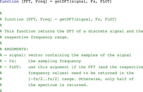
If the concept of negative frequency is introduced, it can be equivalently stated that the DFT frequencies cover the range ![]() , which can be useful for visualization purposes. In the following example, (getDFT()), this is achieved by a call to the fftshift() function, which is fed with the DFT coefficients of the signal. The getDFT() function returns the magnitude of the DFT coefficients, along with the corresponding frequencies (in Hz). Its standard input arguments are the signal and the sampling rate. If a third argument is provided, the function additionally returns the DFT coefficients arranged in the range
, which can be useful for visualization purposes. In the following example, (getDFT()), this is achieved by a call to the fftshift() function, which is fed with the DFT coefficients of the signal. The getDFT() function returns the magnitude of the DFT coefficients, along with the corresponding frequencies (in Hz). Its standard input arguments are the signal and the sampling rate. If a third argument is provided, the function additionally returns the DFT coefficients arranged in the range ![]() , otherwise, only the ‘positive’ part of the spectrum is returned.
, otherwise, only the ‘positive’ part of the spectrum is returned.
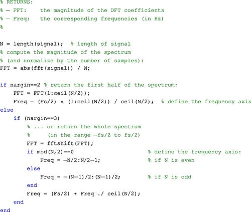
The fftExample() function demonstrates how to call getDFT() by generating a sum of sinusoidal signals with frequencies provided by the user. In the body of the fftExample() m-file, function getDFT() is called twice to compute the spectrum of the generated signal in the two frequency ranges that were described earlier. The time duration of the resulting signal is provided as an input argument to the function.
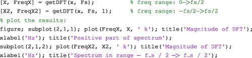
To call the fftExample() function, type:
![]()
The code generates a signal consisting of three tones at 200, 500, and 1200 Hz. The sampling rate is 8 kHz and the signal duration is 0.5 s. The output of the function is plotted in Figure 3.1. The peaks of the magnitude of the spectrum correspond to the three frequencies of the signal.
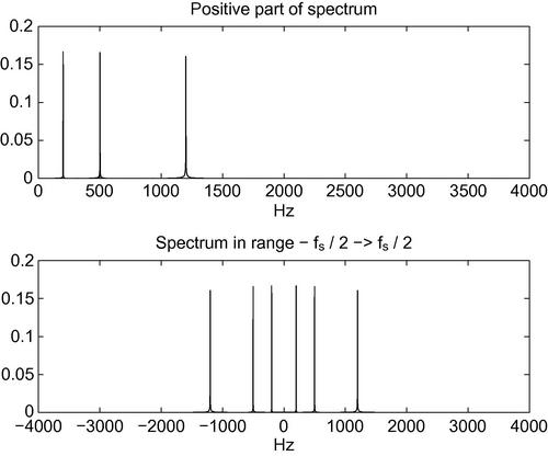
Figure 3.1 Plots of the magnitude of the spectrum of a signal consisting of three frequencies at 200, 500, and 1200 Hz. The sampling frequency is 8 kHz. The frequency ranges on the horizontal axes are [−4 to +4] kHz and [0–4] kHz, respectively.
The next example (fftSNR()) demonstrates the impact of noise on the spectrum of a signal. The function starts by generating a sum of sinusoids as it was done in the previous example. At a second step, Gaussian noise is added to the signal. The signal-to-noise ratio (SNR) is approximately 15 dB and is a user-defined parameter. In the end, the magnitude of the spectrum of both the clean and noisy signals are computed and plotted in decibels.
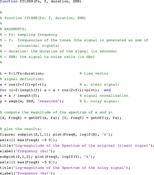
To call fftSNR() type:
![]()
The output of this example is plotted in Figure 3.2.
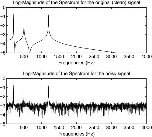
Figure 3.2 A synthetic signal consisting of three frequencies is corrupted by additive noise. The spectra of the original and the noisy signals are plotted (the SNR is 15 dB).
3.2 The Short-Time Fourier Transform
The goal of the Short-Time Fourier Transform (STFT) is to break the signal into possibly overlapping frames using a moving window technique and compute the DFT at each frame. Therefore, the STFT falls in the category of short-term processing techniques (see also Section 2.7). As has already been explained, the length of the moving window plays an important role because it defines the frequency resolution of the spectrum, given the sampling frequency. Longer windows lead to better frequency resolution at the expense of decreasing the quality of time resolution. On the other hand, shorter windows provide a more detailed representation in the time domain, but, in general, lead to poor frequency resolution. In audio analysis applications, the short-term window length usually ranges from 10 to 50 ms. The MPEG7 audio standard recommends that it is a multiple of 10 ms [7].
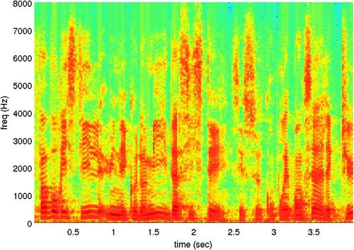
If the DFT coefficients of each frame are placed into a separate column of a matrix, the STFT can be represented as a matrix of coefficients, where the column index represents time and the row index is associated with the frequency of the respective DFT coefficient. If the magnitude of each coefficient is computed, the resulting matrix can be treated as an image and, as a result, it can be visualized. This image is known as the spectrogram of the signal and presents the evolution of the signal in the time-frequency domain. To generate the spectrogram, we can use the magnitude or the squared magnitude of the STFT coefficients on a linear or logarithmic scale (dB). In MATLAB, the spectrogram of a signal is implemented in the spectrogram() function, which can plot the spectrogram and return the matrix of STFT coefficients, along with the respective time and frequency axes. In this book, we will mainly use the spectrogram as a visualization tool. The STFT coefficients will be extracted, when required, by means of a more general function that we have developed for short-term processing purposes. In Figure 3.3, we present an example of a spectrogram for a speech signal.
It is also important to note that before the computation of the DFT coefficients takes place, each frame is usually multiplied on a sample basis with a window function, which aims at attenuating the endpoints of the frame while preserving the signal around the center of the frame. Popular windows have been implemented by MATLAB in the hamming(), hann(), and blackman() m-files. Each function creates a symmetric window based on a different formula.
We are now revisiting the issue of frequency resolution with an example that revolves around the STFT of two frequency-modulated signals. Before we proceed with the example, remember that, on a frame basis, the distance (in Hz) between two successive DFT coefficients is equal to ![]() , where
, where ![]() is the sampling frequency and
is the sampling frequency and ![]() is the number of samples of the frame. The frequency resolution determines when two close frequencies will be distinguishable in the spectrum of the signal. For a fixed sampling rate,
is the number of samples of the frame. The frequency resolution determines when two close frequencies will be distinguishable in the spectrum of the signal. For a fixed sampling rate, ![]() , in order to improve the DFT resolution, we need to increase the length of the short-term frame. However, as it has already been explained, the price to pay is decreased time resolution. Our example creates the following two synthetic signals:
, in order to improve the DFT resolution, we need to increase the length of the short-term frame. However, as it has already been explained, the price to pay is decreased time resolution. Our example creates the following two synthetic signals:
![]()
Each signal is frequency modulated. Consider for example the first equation: the term ![]() creates a 1 Hz signal modulation, which has the effect that the frequency of the tone at 500 Hz exhibits a variation of 200 Hz. The resulting synthetic signal is 2 s long. In this experiment, the sampling frequency is 2 kHz. At the final stage, we create the sum of the two individual signals:
creates a 1 Hz signal modulation, which has the effect that the frequency of the tone at 500 Hz exhibits a variation of 200 Hz. The resulting synthetic signal is 2 s long. In this experiment, the sampling frequency is 2 kHz. At the final stage, we create the sum of the two individual signals:
![]()
We therefore expect that, at each frame, two frequencies should be present, separated by 90 Hz. We now generate the spectrogram of ![]() for three different short-term frame lengths, namely 100, 50, and 10 ms, which correspond to the frequency resolutions of 10, 20, and 100 Hz, respectively. Figure 3.4 presents the generated spectrograms. In the third spectrogram, the frequency resolution (100 Hz) is incapable of distinguishing between the two frequencies, which appear as a single wide band. On the contrary, the frequency resolution of 10 Hz (first spectrogram) separates the two frequencies (which differ by
for three different short-term frame lengths, namely 100, 50, and 10 ms, which correspond to the frequency resolutions of 10, 20, and 100 Hz, respectively. Figure 3.4 presents the generated spectrograms. In the third spectrogram, the frequency resolution (100 Hz) is incapable of distinguishing between the two frequencies, which appear as a single wide band. On the contrary, the frequency resolution of 10 Hz (first spectrogram) separates the two frequencies (which differ by ![]() ), but it fails to follow accurately the time evolution of the signal. It turns out that the best choice is the
), but it fails to follow accurately the time evolution of the signal. It turns out that the best choice is the ![]() frame length, which provides the best trade-off between frequency and time resolution.
frame length, which provides the best trade-off between frequency and time resolution.

Figure 3.4 Spectrograms of a synthetic, frequency-modulated signal for three short-term frame lengths. The best result is achieved by the second spectrogram, because it provides a good trade-off between frequency and time resolution. On the contrary, the first short-term frame length leads to low time resolution, while the third frame length decreases frequency resolution.
3.3 Aliasing in More Detail
The aliasing effect was introduced in Section 2.1. We are now revisiting the aliasing phenomenon with an example involving synthetic signals and through the adoption of frequency representations. Remember that aliasing occurs when the sampling rate is insufficient with respect to the frequency range of the signal, and that, according to the Nyquist theorem, the sampling frequency must be at least twice the highest frequency of the signal to be sampled. From a theoretical point of view, the process of sampling an analog signal creates a discrete-time signal whose frequency representation is a superposition of an infinite number of copies of the Fourier transform of the original signal, where each copy is centered at an integer multiple of the sampling frequency [8–10]. This is presented in Figure 3.5. The second part of the figure displays the spectrum of a sampled signal when the sampling frequency is higher than the Nyquist rate. It can be observed that the shifted copies of the analog spectrum of the first part of the figure are non-overlapping. On the contrary, the third part demonstrates the case of insufficient sampling rate. It can be seen that the replicas of the analog spectrum are now overlapping, giving rise to the aliasing phenomenon.
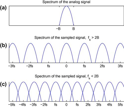
Figure 3.5 Spectrum representations of (a) an analog signal, (b) a sampled version when the sampling frequency exceeds the Nyquist rate, and (c) a sampled version with insufficient sampling frequency. In the last case, the shifted versions of the analog spectrum are overlapping, hence the aliasing effect.
Figure 3.6 presents the aliasing phenomenon for a simple signal. The signal ![]() consists of a sum of three tones at frequencies 200, 500, and 3000 Hz. Based on the Nyquist theorem, the minimum acceptable sampling rate is
consists of a sum of three tones at frequencies 200, 500, and 3000 Hz. Based on the Nyquist theorem, the minimum acceptable sampling rate is ![]() . The figure presents the spectra of the sampled signal when the sampling frequency is
. The figure presents the spectra of the sampled signal when the sampling frequency is ![]() and
and ![]() , respectively. The second sampling frequency causes an aliasing effect: the
, respectively. The second sampling frequency causes an aliasing effect: the ![]() tone fails to be preserved in the discrete-time signal representation and its alias appears as a new frequency at
tone fails to be preserved in the discrete-time signal representation and its alias appears as a new frequency at ![]() .
.

Figure 3.6 Spectral representations of the same three-tone (200, 500 and 3000 Hz) signal for two different sampling frequencies (8 kHz and 4 kHz). The 4 kHz rate generates an aliasing effect because the 3KHz frequency vanishes and its alias at 1KHz appears instead.
3.4 The Discrete Cosine Transform
Another transform that has been widely used in the field of signal processing is the Discrete Cosine Transform (DCT) [11,5]. It is a purely real transform, because, unlike the DFT, which uses complex exponentials as its basis functions, the DCT expresses a finite duration signal as a weighted sum of cosines (real functions). The DCT has been very popular in the development of coding applications, especially in the case of two-dimensional signals (images).
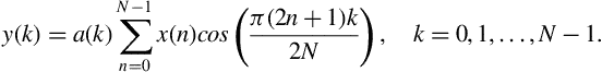
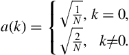
Let ![]() be a discrete-time signal of finite duration. Its DCT is defined as
be a discrete-time signal of finite duration. Its DCT is defined as
We observe that Eq. (3.4) generates ![]() DCT coefficients,
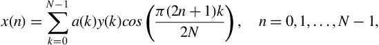
DCT coefficients, ![]() , which will serve as the weights of the basis functions in the following equation that defines the inverse DCT:
, which will serve as the weights of the basis functions in the following equation that defines the inverse DCT:
where
An interesting property of the DCT, which leads to computationally efficient implementations, is that it can be expressed as a product of matrices, i.e. ![]() , where
, where ![]() has real elements and
has real elements and ![]() . In the MATLAB programming environment, the DCT has been implemented in the dct() function of the Signal Processing Toolbox.
. In the MATLAB programming environment, the DCT has been implemented in the dct() function of the Signal Processing Toolbox.
Another interesting feature of the DCT is that it provides very good information—packing options. This is why the two-dimensional DCT has been embedded in the JPEG image compression standard. The one-dimensional DCT has also been adopted by audio coding standards. For example, the MPEG1-Layer III (MP3) standard uses a modified DCT. Further to its adoption by compression techniques, the DCT has been also employed by various feature extraction algorithms. An outstanding example is the adoption of the inverse DCT as the last processing stage in the extraction of the Mel-Frequency Cepstrum Coefficients (MFCCs) from the audio signal [8]. More details on this matter can be found in Section 4.4.5, in the following chapter.
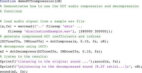
In this section, we will present an example that demonstrates the basic ideas behind the DCT-based compression and decompression of an audio signal. Our simple compression-decompression scheme goes through the following steps:
• The signal is split into non-overlapping windows. The length of the moving window is set equal to ![]() .
.
• For each window, the DCT is computed.
• The DCT coefficients are sorted in descending order based on their amplitude. The DCT coefficients which correspond to the ![]() of highest amplitude values are preserved along with their indices. The remaining DCT coefficients are set to zero.
of highest amplitude values are preserved along with their indices. The remaining DCT coefficients are set to zero.
• The inverse DCT is applied on the modified sequence of DCT coefficients. The result is a real-valued, time-domain signal, which has preserved the dominant characteristics of the original signal and has discarded unnecessary detail.
The dctCompress() function implements the compression steps of the above scheme. The DCT coefficients that survive at each frame along with the respective indices are stored as rows of data in two separate matrices. To decompress the signal, the inverse procedure is executed: the DCT coefficients at each row of the respective matrix are used to compute the inverse DCT. The decompression stage has been implemented in the dctDecompress() function. The following piece of code demonstrates how to use functions dctCompress() and dctDecompress(), given an input signal. Part of the example file diarizationExample.wav has been used here, which is also included in the library that comes with this book. The only input argument of this demo function is the required compression ratio.
3.5 The Discrete-Time Wavelet Transform
The goal of the Discrete-Time Wavelet Transform (DTWT) is to provide a multiresolution analysis framework for the study of signals. The term multiresolution refers to the fact that the signal is split into a hierarchy of signal versions of increasing detail. The original signal can be reconstructed from its versions by means of a weighting scheme, which is defined by the inverse DTWT. The theory of the DTWT is quite complicated and can be approached from different perspectives. For example, it is common to present the DTWT from the point of view of tree-structured filter banks, which in turn requires that the reader is familiar with filter theory. In this section we will only provide the analysis and synthesis equations of the DTWT and its inverse, following the presentation that we also adopted for the DFT and the DCT. We will comment on the respective equations and then we will explain the steps of multiresolution analysis using MATLAB code.
To begin with, the DTWT is defined as
where index ![]() represents the analysis (resolution) level,
represents the analysis (resolution) level, ![]() is the index of the DTWT coefficients at the
is the index of the DTWT coefficients at the ![]() th level, and the
th level, and the ![]() s are appropriately defined functions. The inverse DTWT performs a perfect reconstruction of the original signal and it is given by the equation
s are appropriately defined functions. The inverse DTWT performs a perfect reconstruction of the original signal and it is given by the equation
where the ![]() s are the basis functions at the
s are the basis functions at the ![]() th level. An important issue is that the functions at each analysis level stem from an appropriately defined mother function:
th level. An important issue is that the functions at each analysis level stem from an appropriately defined mother function:
where ![]() if
if ![]() if
if ![]() and
and ![]() is the mother sequence of the
is the mother sequence of the ![]() th level. It can be seen that all the functions of an analysis level are shifted versions of the mother function. Similarly, for the inverse transform,
th level. It can be seen that all the functions of an analysis level are shifted versions of the mother function. Similarly, for the inverse transform,
where ![]() if
if ![]() if
if ![]() and
and ![]() is the mother sequence of the
is the mother sequence of the ![]() th level. You have probably guessed that if the reconstruction of the original signal takes into account less than
th level. You have probably guessed that if the reconstruction of the original signal takes into account less than ![]() levels, then an approximate (coarse) version of the original signal will be made available.
levels, then an approximate (coarse) version of the original signal will be made available.
In order to get a better understanding of the DTWT and its inverse, let us follow a hierarchical decomposition of a signal using a series of MATLAB commands. MATLAB provides the functionality that we need in the Wavelet Toolbox. Specifically, we will use the dwt() function for splitting the signal into two components and the idwt() function for the reconstruction stage. First of all, we need to load a signal. To this end, we select a segment, 1024 samples long, drawn from the previously used diarizationExample.wav file.
![]()
Then we decompose the signal into two components:
![]()
The second input argument specifies the mother function of the analysis stage. The first output argument, ![]() , is the vector of DTWT coefficients of the coarse analysis level and the second output argument,
, is the vector of DTWT coefficients of the coarse analysis level and the second output argument, ![]() , contains the coefficients, which capture the detail of the signal. Note that the length of each output signal is half the length of the input signal
, contains the coefficients, which capture the detail of the signal. Note that the length of each output signal is half the length of the input signal ![]() . We can now plot the two signals:
. We can now plot the two signals:
The next step is to further decompose the coarse approximation, ![]() , into two signals,
, into two signals, ![]() and
and ![]() :
:
![]()
This time, vectors ![]() and
and ![]() contain 256 analysis coefficients. We can now plot
contain 256 analysis coefficients. We can now plot ![]() , and
, and ![]() in a single figure:
in a single figure:
In other words, we have performed a two-stage analysis of the original signal. We will now proceed with the inverse operation, i.e. we will reconstruct the signal in two stages. For the first reconstruction stage, type:
![]()
The reconstructed signal, ![]() , is 512 samples long. To proceed with the next reconstruction stage, type:
, is 512 samples long. To proceed with the next reconstruction stage, type:
![]()
Note that if we use zeros instead of the ![]() signal, this will mean that we are not interested in the detail that the
signal, this will mean that we are not interested in the detail that the ![]() signal carries. If this is desirable, we can type:
signal carries. If this is desirable, we can type:
![]()
If you plot ![]() and the original signal in the same figure, you will readily observe that their differences are really minor. In practice, this means that we were right to ignore the detail in the
and the original signal in the same figure, you will readily observe that their differences are really minor. In practice, this means that we were right to ignore the detail in the ![]() signal. The respective SNR (signal-to-noise ratio) will reveal the same observation (see also Exercise 7, which is on the computation of SNR).
signal. The respective SNR (signal-to-noise ratio) will reveal the same observation (see also Exercise 7, which is on the computation of SNR).
3.6 Digital Filtering Essentials
The goal of this section is to provide a gentle introduction to the design of digital filters, focusing on reproducible MATLAB examples. Digital filters are important building blocks in numerous contemporary processing systems that perform diverse operations, ranging from quality enhancement to multiresolution analysis. The interested reader may consult several textbooks in the field, which provide a detailed treatment of the subject from both a theoretical and implementation perspective, e.g. [8,1,12,13].
To begin with, consider the following equation, which describes the signal ![]() at the output of a system as a function of the signal
at the output of a system as a function of the signal ![]() at its input:
at its input:
where ![]() is a constant and
is a constant and ![]() . Equation (3.11) describes a filter, i.e. a system whose output at the
. Equation (3.11) describes a filter, i.e. a system whose output at the ![]() th discrete-time instant is computed as a function of the current input sample,
th discrete-time instant is computed as a function of the current input sample, ![]() and a weighted version of the previous input sample,
and a weighted version of the previous input sample, ![]() . Now, let us assume that the following signal is given as input to the filter:
. Now, let us assume that the following signal is given as input to the filter:
This signal is also known as the unit impulse sequence. It is straightforward to compute the output of the system for this simple signal:

where ![]() . The response of the system to the unit impulse sequence is known as the impulse response of the system. The impulse response is a signal that offers an alternative representation of the system. In this case, the impulse response becomes zero after the second sample
. The response of the system to the unit impulse sequence is known as the impulse response of the system. The impulse response is a signal that offers an alternative representation of the system. In this case, the impulse response becomes zero after the second sample ![]() . When this type of behavior is observed, we are dealing with a Finite Impulse Response (FIR) filter (system). In the more general case, a FIR system is described by the equation:
. When this type of behavior is observed, we are dealing with a Finite Impulse Response (FIR) filter (system). In the more general case, a FIR system is described by the equation:
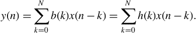
A quick inspection of Eq. (3.14) reveals that the output of a FIR system is always a function of the current and past samples of the input signal. Number ![]() is known as the order of the filter.
is known as the order of the filter.
The DFT of the impulse response is called the frequency response of the filter. Given that the impulse response of the FIR filters becomes zero after a finite number of samples, it follows that, if we want to study the frequency response of a FIR system with sufficient frequency detail, we need to resort to the technique of zero padding that was described in the context of the DFT transform.
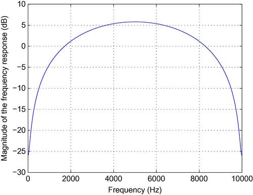
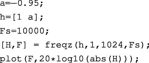
Assuming that our filter operates at a sampling frequency of ![]() , we can type the following commands to generate and plot the magnitude of its frequency response:
, we can type the following commands to generate and plot the magnitude of its frequency response:
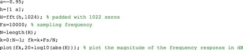
In the above lines of code the ![]() parameter was set equal to
parameter was set equal to ![]() . As a result, on a dB scale, the frequency response is negative for the low-frequency range [0–1700] Hz (approximately) and positive for frequencies higher than
. As a result, on a dB scale, the frequency response is negative for the low-frequency range [0–1700] Hz (approximately) and positive for frequencies higher than ![]() , as shown in Figure 3.7. In other words, the filter attenuates the low-frequency range and amplifies the frequencies in the range [1700–5000] Hz. This type of frequency response is particularly useful as a preprocessing stage when the human voice is recorded over a microphone, because most microphones tend to emphasize low frequencies. Our filter has the inverse effect: it emphasizes the high frequencies (if
, as shown in Figure 3.7. In other words, the filter attenuates the low-frequency range and amplifies the frequencies in the range [1700–5000] Hz. This type of frequency response is particularly useful as a preprocessing stage when the human voice is recorded over a microphone, because most microphones tend to emphasize low frequencies. Our filter has the inverse effect: it emphasizes the high frequencies (if ![]() ), hence the name pre-emphasis filter.
), hence the name pre-emphasis filter.
FIR systems fall in the broader category of Linear Time Invariant (LTI) systems. The linear property defines that a linear combination of inputs will produce the same linear combination of outputs. For example, if our simple filter is fed with the signal ![]() , the output will be:
, the output will be:

where ![]() and
and ![]() are the signals at the output of the filter when the input signals are
are the signals at the output of the filter when the input signals are ![]() and
and ![]() , respectively. The property of time invariance defines that a shifted version of the input will produce a shifted version of the output by the same amount of time shift.
, respectively. The property of time invariance defines that a shifted version of the input will produce a shifted version of the output by the same amount of time shift.
A different category of filters can be designed if the right side of the input-output equation includes past values of the output:
If at least one ![]() is nonzero, Eq. (3.16) describes the category of Infinite Impulse Response (IIR) filters (otherwise it reverts to a description of a FIR filter). Due to the infinite length of their impulse response, we need the recurrence relation of Eq. (3.16) to compute the output of IIR filters, i.e. it no longer makes sense to use a summation like the one in Eq. (3.14).
is nonzero, Eq. (3.16) describes the category of Infinite Impulse Response (IIR) filters (otherwise it reverts to a description of a FIR filter). Due to the infinite length of their impulse response, we need the recurrence relation of Eq. (3.16) to compute the output of IIR filters, i.e. it no longer makes sense to use a summation like the one in Eq. (3.14).
Another important categorization of digital filters is based on the shape of the frequency response. Specifically, the filters can be categorized in the lowpass, bandpass, highpass, and stopband categories. Basically, the names indicate the frequency range (passband) where the magnitude of the frequency response of the filter is expected to be equal to unity (on a linear scale) or ![]() (on a logarithmic scale). For example, the term lowpass means that the filter is expected to leave unaltered all frequencies in the range
(on a logarithmic scale). For example, the term lowpass means that the filter is expected to leave unaltered all frequencies in the range ![]() , where
, where ![]() marks the end of the passband. In practice, the transition from the passband to the stopband is not sharp and requires that a transition region exists. Therefore, during the design of a lowpass digital filter we specify the boundaries of the transition region instead of the single frequency,
marks the end of the passband. In practice, the transition from the passband to the stopband is not sharp and requires that a transition region exists. Therefore, during the design of a lowpass digital filter we specify the boundaries of the transition region instead of the single frequency, ![]() . We also specify the desirable attenuation in the stopband (in dB) and the allowable change in the passband (in dB). In other words, the set of specifications aims at providing an approximation of the ideal situation. Unfortunately, unless the order of the filter is very high, it is very hard to satisfy all the specifications. MATLAB provides some interesting tools that the designer of filters can use in order to experiment with various filter specifications (e.g. the fdatool which is presented in the next section).
. We also specify the desirable attenuation in the stopband (in dB) and the allowable change in the passband (in dB). In other words, the set of specifications aims at providing an approximation of the ideal situation. Unfortunately, unless the order of the filter is very high, it is very hard to satisfy all the specifications. MATLAB provides some interesting tools that the designer of filters can use in order to experiment with various filter specifications (e.g. the fdatool which is presented in the next section).
3.7 Digital Filters in MATLAB
Filtering is implemented in the MATLAB environment in the built-in filter() function. The syntax of the function is:
![]()
The input arguments are:
For example, to filter a signal that is stored in vector ![]() through the pre-emphasis filter
through the pre-emphasis filter ![]() , type:
, type:
![]()
Another useful function, with input arguments that follow the rationale of the filter() function is the freqz() function, which generates the frequency response of a filter, given the coefficients of Eq. (3.16). For example, the following commands generate and plot the frequency response of our pre-emphasis filter:
The fdatool of the Signal Processing Toolbox of MATLAB provides a graphical user interface (GUI) to facilitate the design and analysis of digital filters. The user is allowed to describe the frequency response of the filter via a set of specifications. After the filter has been designed, the fdatool can be used to export the resulting filter coefficients (i.e. the a and b vectors) to the MATLAB workspace, to a MAT file, or to MATLAB code that can reproduce the filter design.
An alternative way to design a digital filter in MATLAB is by using the fdesign object of the Signal Processing Toolbox. Similar to the fdatool, the user again provides the filter specifications, i.e. type of filter, the critical frequencies and respective attenuations, etc.
The following example begins with the generation of a synthetic signal that consists of three frequencies. Then, it creates a lowpass filter and applies it on the generated signal. The spectrograms of the initial and the filtered signal, along with the frequency response of the designed filter are shown in Figure 3.8.


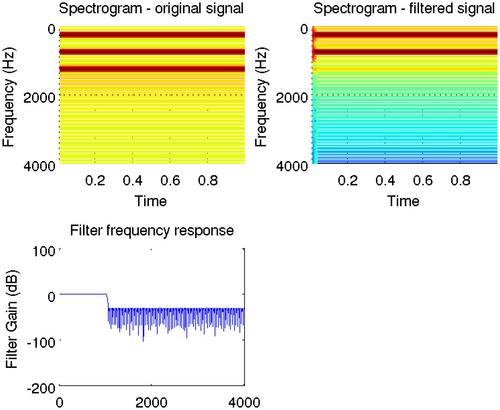
Figure 3.8 An example of the application of a lowpass filter on a synthetic signal consisting of three tones. The spectrogram of the output of the filter reveals that the highest tone has been filtered out.
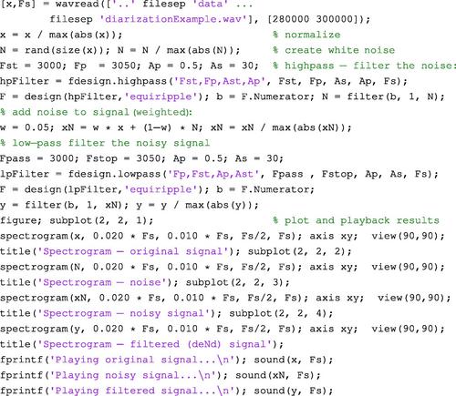
Finally, let us present a very simple example of a speech denoising technique, which goes through the following steps:
1. Loads a speech signal from a WAVE file.
2. Generates a white noise signal of equal duration with the speech signal.
3. Uses a highpass filter to preserve the frequencies of the noise above 3 kHz.
4. Adds the filtered noise to the original signal.
5. Denoises the signal with a lowpass filter.
6. Reproduces all three signals and plots their spectrograms.
The MATLAB code that implements this simple denoising approach is the following (stored in the demoFilter2() m-file of the library):
During the playback of the noisy signal, the speech signal can be hardly perceived, whereas this is not the case with the filtered signal. However, note that this demo is only presenting a naive denoising procedure. In a real-world scenario the noise is not expected to be limited to high frequencies and therefore more sophisticated denoising approaches need to be adopted. Figure 3.9 illustrates the results of this filtering process for a speech signal example.
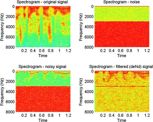
Figure 3.9 Example of a simple speech denoising technique applied on a segment of the diarizationExample.wav file, found in the data folder of the library of the book. The figure represents the spectrograms of the original signal, the high-frequency noise, the noisy signal, and the final filtered signal.
3.8 Exercises
1. (D3) Use the fdesign object to design a bandpass filter that attenuates all frequencies outside the range ![]() . Apply it on audio signals of your choice, plot the spectrograms of the results, and reproduce the respective sounds.
. Apply it on audio signals of your choice, plot the spectrograms of the results, and reproduce the respective sounds.
2. (D5) Use the GUIDE tool of MATLAB to create a GUI that implements the following requirements:
(a) When a button is pressed, the GUI records 2 s of audio (see also Section 2.6), using MATLAB’s audiorecorder, as it was explained in Section 2.6.2. The recorded signal is stored in a temporary WAV file.
(b) Generates a FIR bandpass filter using the fdesign tool. The frequencies that specify the passband of the filter are provided by the user by means of two sliders.
(c) Uses a variant of the stpFile() function (see also Section 2.7) to apply the bandpass filter on each short-term window of the recorded signal.
(d) When a ‘play’ button is pressed, the filtered signal is reproduced.
3. (D1) We are given the signal ![]() . How many zeros need to be padded at the end of the signal, so that the frequency resolution of the DFT is
. How many zeros need to be padded at the end of the signal, so that the frequency resolution of the DFT is ![]() , assuming that the sampling frequency is
, assuming that the sampling frequency is ![]() ?
?
4. (D3) Assume that we want to design a pre-emphasis filter, so that the magnitude of its frequency response is equal to ![]() on a linear scale. Assuming that the sampling frequency is
on a linear scale. Assuming that the sampling frequency is ![]() , what value should we use for the
, what value should we use for the ![]() parameter in the equation
parameter in the equation ![]() ?
?
5. (D2) The analog signal ![]() is sampled at
is sampled at ![]() . How many samples are necessary so that the frequency resolution of the DFT is sufficient to distinguish the two frequencies in the spectrum of the signal?
. How many samples are necessary so that the frequency resolution of the DFT is sufficient to distinguish the two frequencies in the spectrum of the signal?
6. (D2) The analog signal ![]() is sampled with a
is sampled with a ![]() sampling frequency. What is the resulting discrete-time signal?
sampling frequency. What is the resulting discrete-time signal?
7. (D3) Let ![]() be a signal and
be a signal and ![]() its reconstruction. The difference between the original signal and its reconstruction can be quantified by the signal-to-noise ratio (SNR), which is defined as:
its reconstruction. The difference between the original signal and its reconstruction can be quantified by the signal-to-noise ratio (SNR), which is defined as:
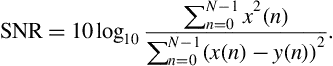
Implement a function that computes the SNR given a signal and its reconstruction. Compute the SNR of the DCT compression scheme (Section 3.4) and DTWT reconstruction procedure. Use the speech segment of the diarizationExample.wav file, as in Section 3.5. You can also experiment with different values of the compression ratio to investigate how this parameter affects the respective SNR.