
Audio Segmentation
Abstract
This chapter focuses on a vital stage of audio analysis, the audio segmentation stage, which focuses on splitting an uninterrupted audio signal into segments of homogeneous content. The chapter describes two general categories of audio segmentation: those that employ supervised knowledge and those that are unsupervised or semi-supervised. In this presentation context, certain specific segmentation tasks are presented, e.g., silence removal and speaker diarization.
Keywords
Audio segmentation
Fixed-window segmentation
Probability smoothing
Silence removal
Signal change detection
Speaker diarization
Clustering
Unsupervised learning
Semi-supervised learning
Segmentation is a processing stage that is of vital importance for the majority of audio analysis applications. The goal is to split an uninterrupted audio signal into segments of homogeneous content. Due to the fact that the term ‘homogeneous’ can be defined at various abstraction layers depending on the application, there exists an inherent difficulty in providing a global definition for the concept of segmentation.
For example, if our aim is to break a radio broadcast of classical music into homogeneous segments, we would expect that, in the end, each segment will contain either speech or classical music (or silence). In this case, the definition of the term homogeneous is based on the audio types that we expect to encounter in the audio stream and we demand that each segment at the output of the segmentation stage consists of only one audio type [24]. Obviously, a different definition is necessary, when we know that we are processing a speech stream by means of a diarization system which aims at determining ‘who spoke when?’ [64]. In this case, the definition of homogeneity is tied with the identity of the speaker, i.e. we can demand that each segment contains the voice of a single speaker. As a third example, consider a music signal of a single wind instrument (e.g. a clarinet). The output of the segmentation stage can be the sequence of individual notes (and pauses) in the music stream. At a more abstract level, we might need to develop a segmentation algorithm, which can break the audio stream of a movie into audio scenes, depending on whether violent audio content is present or not [20].
In this chapter, we first focus on segmentation methods that exploit prior knowledge of the audio types which are involved in the audio stream. These methods are described in Section 6.1 and embed classification decisions in the segmentation algorithm. Section 6.2 describes methods that do not make use of prior knowledge. The methods of this second category either detect stationarity changes in the content of the signal or use unsupervised clustering techniques to divide the signal into segments, so that segments of the same audio type are clustered together.
6.1 Segmentation with Embedded Classification
Several algorithms evolve around the idea of executing the steps of segmentation and classification, jointly [60,23,24]. A simple approach is to split the audio stream into fixed-size segments, classify each segment separately, and merge successive segments of the same audio type at a post-processing stage. Alternatively, if fixed-size splitting is abandoned and the segmentation procedure becomes dynamic, the classifier can be embedded in the segmentation decisions [24]. In other words, the endpoints of the segments can be dynamically determined by taking into account the potential decision of the classifier on the candidate segments. In both cases, the output of the segmentation stage is a sequence of (classified) homogeneous audio segments. The nature of these methods demands that a trained classifier is available, which can be a major restriction depending on the application context. Unfortunately, a trained classifier can often be a luxury because the training data may not be available or the audio data types may not be fixed in advance. These demands call for an ‘unsupervised’ approach to segmentation, as will be explained in Section 6.2.
6.1.1 Fixed-Window Segmentation
Fixed-window segmentation is a straightforward approach to segmenting an audio stream if a trained classifier is available. The signal is first divided into (possibly) overlapping mid-term segments (e.g. 1 s long) and each segment is classified separately to a predefined set of ![]() audio classes. As a result, a sequence of hard classifications decisions (audio labels),
audio classes. As a result, a sequence of hard classifications decisions (audio labels), ![]() is generated at the output of this first stage, where
is generated at the output of this first stage, where ![]() is the number of mid-term segments. The extracted sequence of audio labels is then smoothed at a second (post-processing) stage, yielding the final segmentation output, i.e. a sequence of pairs of endpoints (one pair per detected segment) along with the respective audio (class) labels (Figure 6.2).
is the number of mid-term segments. The extracted sequence of audio labels is then smoothed at a second (post-processing) stage, yielding the final segmentation output, i.e. a sequence of pairs of endpoints (one pair per detected segment) along with the respective audio (class) labels (Figure 6.2).
Note that, instead of hard classification decisions, the output of the first stage can be a set of soft outputs, ![]() , for the
, for the ![]() th segment. The soft outputs can be interpreted as the estimates of the posterior probabilities of the classes,
th segment. The soft outputs can be interpreted as the estimates of the posterior probabilities of the classes, ![]() , given the feature vector,
, given the feature vector, ![]() , that represents the mid-term segment (obviously,
, that represents the mid-term segment (obviously, ![]() ). Therefore, depending on the output of the first stage, we can broadly classify the techniques of the second stage in two categories:
). Therefore, depending on the output of the first stage, we can broadly classify the techniques of the second stage in two categories:
• Naive merging techniques: the key idea is that if successive segments share the same class label, then they can be merged to form a single segment (Section 6.1.1.1).
• Probability smoothing techniques: if the adopted classification scheme has a soft output, then it is possible to apply more sophisticated smoothing techniques on the sequence that has been generated at the output of the first stage. Section 6.1.1.2 explains in detail a smoothing technique that is capable of processing a sequence of soft outputs and presents its application on an audio stream.
Figure 6.1 provides a schematic description of the post-processing stage. Irrespective of the selected post-segmentation technique, the output is a sequence of pairs of endpoints, ![]() and respective class labels,
and respective class labels, ![]() , where
, where ![]() is the final number of segments. Note that, throughout this chapter we will use the terms ‘post-processing,’ ‘post-segmentation,’ and ‘smoothing’ interchangeably when we refer to the second processing stage of the segmenter.
is the final number of segments. Note that, throughout this chapter we will use the terms ‘post-processing,’ ‘post-segmentation,’ and ‘smoothing’ interchangeably when we refer to the second processing stage of the segmenter.

Figure 6.1 Post-segmentation stage: the output of the first stage can be (a) a sequence of hard classification decisions, ![]() ; or (b) a sequence of sets of posterior probability estimates,
; or (b) a sequence of sets of posterior probability estimates, ![]() . The
. The ![]() s provide temporal information, i.e. refer to the center of each fixed-term segment. The output is a sequence of pairs of endpoints,
s provide temporal information, i.e. refer to the center of each fixed-term segment. The output is a sequence of pairs of endpoints, ![]() and respective class labels
and respective class labels ![]() , where
, where ![]() is the final number of segments.
is the final number of segments.
6.1.1.1 Naive Merging
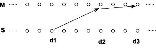
This simple procedure assumes that a sequence of audio labels (hard classification decisions) has been generated by the first stage of the segmenter. The only action that is performed by the post-segmentation stage is to merge successive mid-term segments of the same class label in to a single, longer segment. This rationale is illustrated in Figure 6.2, where a binary classification problem of speech vs music has been assumed.
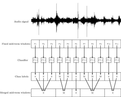
Figure 6.2 Fixed-window segmentation. Each subsequence whose elements exhibit the same hard label merge forming a single segment. ‘S’ and ‘M’ stand for the binary problem of speech vs music.
The post-processing functionality of the naive merging scheme has been implemented in the segmentationProbSeq() m-file of the MATLAB toolbox provided with the book. Note that this function needs to be called after the mtFileClassification() function, which generates a set of estimates of the posterior class probabilities for each mid-term window. At each segment, function segmentationProbSeq() determines the class label based on the maximum probability and then proceeds with the merging procedure. The first input argument of segmentationProbSeq() is a matrix, ![]() , where
, where ![]() corresponds to the estimated probability that the
corresponds to the estimated probability that the ![]() th window belongs to the
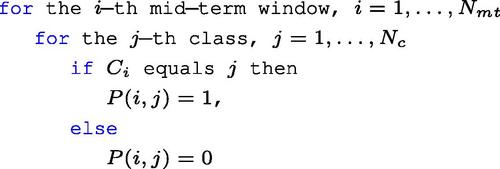
th window belongs to the ![]() th class. If the adopted classifier can only provide a hard decision,
th class. If the adopted classifier can only provide a hard decision, ![]() , for the
, for the ![]() th mid-term window, it is still easy to generate the input matrix,
th mid-term window, it is still easy to generate the input matrix, ![]() , using the following rule (given in pseudocode):
, using the following rule (given in pseudocode):
In more detail, function segmentationProbSeq() accepts the following arguments:
1. The matrix of probabilities, ![]() , which was described above. It has
, which was described above. It has ![]() rows (equal to the number of fixed mid-term windows) and
rows (equal to the number of fixed mid-term windows) and ![]() columns (equal to the number of classes). Note that in the naive merging mode, only hard decisions are needed, so the segmentationProbSeq() function can simply select from each row the class that corresponds to the maximum probability. Several of the examples in this book use the
columns (equal to the number of classes). Note that in the naive merging mode, only hard decisions are needed, so the segmentationProbSeq() function can simply select from each row the class that corresponds to the maximum probability. Several of the examples in this book use the ![]() -NN classifier, which can provide soft outputs. Of course, there is always the option to use the aforementioned rule for the conversion of the output of any classifier that provides hard decisions to a compatible
-NN classifier, which can provide soft outputs. Of course, there is always the option to use the aforementioned rule for the conversion of the output of any classifier that provides hard decisions to a compatible ![]() -matrix.
-matrix.
2. ![]() : the centers (in seconds) of the corresponding mid-term windows.
: the centers (in seconds) of the corresponding mid-term windows.
3. The total duration of the input signal, which is used to generate the endpoints of the last segment. The example at the end of this section demonstrates how to obtain this quantity.
4. The type of post-segmentation technique: 0 for naive merging and 1 for probability smoothing (see Section 6.1.1.2).
The output of the segmentationProbSeq() function is a ![]() matrix,
matrix, ![]() , whose rows correspond to the endpoints of the detected segments, i.e.
, whose rows correspond to the endpoints of the detected segments, i.e. ![]() marks the beginning of the
marks the beginning of the ![]() th segment and
th segment and ![]() its end. Both quantities are provided in seconds. Furthermore, segmentationProbSeq() returns a vector,
its end. Both quantities are provided in seconds. Furthermore, segmentationProbSeq() returns a vector, ![]() , with the corresponding audio labels. The following code demonstrates how to use the chain of functions mtFileClassification() and segmentationProbSeq() in the context of fixed-window segmentation with a naive post-processing stage. We focus on the binary task of speech-music classification and load the dataset that is stored in the modelSM.mat file.
, with the corresponding audio labels. The following code demonstrates how to use the chain of functions mtFileClassification() and segmentationProbSeq() in the context of fixed-window segmentation with a naive post-processing stage. We focus on the binary task of speech-music classification and load the dataset that is stored in the modelSM.mat file.

The reason that function segmentationProbSeq() operates on a matrix of probabilities instead of a sequence of hard decisions, is that we want to provide a single m-file for both post-processing techniques. Therefore, as the reader understands, this is just a software engineering issue and all that is needed for the naive merger to operate is an intermediate conversion of matrix ![]() to hard labels, as explained above.
to hard labels, as explained above.
6.1.1.2 Probability Smoothing
The post-segmentation scheme of the previous section merges successive mid-term windows of the same class label and does not really make use of the soft (probabilistic) output of the classifier, whenever such output is available. On the other hand, if the classification probabilities are exploited, a more sophisticated post-processing scheme can be designed. Consider, for example, a binary classifier of speech vs music embedded in a segmenter and assume that for a mid-term window the classification decision is ‘marginal’ with respect to the estimated probabilities. For instance, if the ![]() -NN classifier is employed with
-NN classifier is employed with ![]() , it could be the case that five neighbors belong to the speech class and the rest of them to the music class. The respective estimates of the posterior probabilities are
, it could be the case that five neighbors belong to the speech class and the rest of them to the music class. The respective estimates of the posterior probabilities are ![]() and
and ![]() , respectively. Although the segment is classified to the speech class, there exists a high probability that a classification error has occurred. In other words, the naive merger of the previous section may have to operate on a noisy sequence of classification decisions. In such situations, the performance of the post-processing stage can be boosted if a smoothing technique is applied on the soft outputs of the classifier.
, respectively. Although the segment is classified to the speech class, there exists a high probability that a classification error has occurred. In other words, the naive merger of the previous section may have to operate on a noisy sequence of classification decisions. In such situations, the performance of the post-processing stage can be boosted if a smoothing technique is applied on the soft outputs of the classifier.
Figure 6.3 is an example of the application of two post-segmentation procedures on the binary classification problem of speech vs music. Figure 6.3a presents the posterior probability estimates for the two classes (speech and music) over time. Figure 6.3b presents the results of the naive merging scheme, and Figure 6.3c refers to the output of a Viterbi-based smoothing technique that will be explained later in the section. The example highlights the fact that the classifier produces marginal decisions near the 20th second of the audio stream because the posterior probabilities of the two classes are practically equal. The simple merging technique treats the respective segment as music. On the other hand, the smoothing approach takes into account the neighboring probabilistic output of the classifier and generates a ‘smoother’ decision as far as the transition among class labels is concerned.

The Viterbi algorithm [65, 66] is a dynamic programming algorithm, which, broadly speaking, is aimed at finding the most likely sequence of states, given a sequence of observations. In the context of segmentation, a Viterbi-based algorithm can be designed to determine the most likely sequence of class labels, given the posterior probability estimations on a segment basis [64, 67]. Further to the given probabilities, the Viterbi-based post-segmentation algorithm also needs as input the prior class probabilities and a transition matrix, ![]() , whose elements,
, whose elements, ![]() , indicate the probability of transition from state
, indicate the probability of transition from state ![]() to state
to state ![]() , i.e. in our case, from class label
, i.e. in our case, from class label ![]() to class label
to class label ![]() (assuming
(assuming ![]() classes in total). The core Viterbi algorithm will be further explained in Chapter 7 because it is also an essential algorithm in the context of temporal modeling and recognition. In this chapter, the key idea of the algorithm is preserved and adopted for the purpose of post-processing.
classes in total). The core Viterbi algorithm will be further explained in Chapter 7 because it is also an essential algorithm in the context of temporal modeling and recognition. In this chapter, the key idea of the algorithm is preserved and adopted for the purpose of post-processing.
Our version of the Viterbi-based post-processing scheme is tailored to the needs of probability smoothing and it is implemented in function viterbiBestPath(). In order to embed the Viterbi-based smoothing procedure in the segmenter, the following initialization steps need to be executed, given a matrix, ![]() , of posterior probability estimations, where
, of posterior probability estimations, where ![]() corresponds to the estimated probability that the
corresponds to the estimated probability that the ![]() th segment belongs to the
th segment belongs to the ![]() th class:
th class:
1. Estimation of the class priors. A simple technique to initialize the class priors is to convert the ![]() matrix to a sequence of hard decisions and subsequently count the frequency of occurrence of each class. The conversion to hard decisions can be simply achieved by selecting from each row the class that corresponds to the highest probability.
matrix to a sequence of hard decisions and subsequently count the frequency of occurrence of each class. The conversion to hard decisions can be simply achieved by selecting from each row the class that corresponds to the highest probability.
2. Estimation of the transition matrix, ![]() . We operate again on the sequence of hard decisions. In order to estimate
. We operate again on the sequence of hard decisions. In order to estimate ![]() , we count the transitions from class
, we count the transitions from class ![]() to class
to class ![]() in the sequence and divide by the total number of transitions from class
in the sequence and divide by the total number of transitions from class ![]() to any class.
to any class.
3. The matrix, ![]() , of probability estimations is directly given as input to the Viterbi-based technique.
, of probability estimations is directly given as input to the Viterbi-based technique.
The complete post-segmentation procedure can be called via function segmentationProbSeq() by setting the input argument ‘method’ equal to 1. This is presented in the following piece of code:
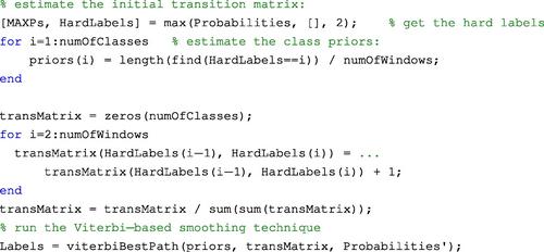
In the end of the above initialization procedure, the ‘labels’ vector contains the sequence of class labels at the output of the Viterbi algorithm. In other words, this vector contains the sequence of class labels that maximizes the Viterbi score given the estimated (observed) class probabilities on a mid-term basis. After the best-class sequence has been generated, the naive merger is applied on the results in order to yield the final sequence of segments.
6.1.1.3 Example: Speech-Silence Segmentation
The ability to detect the useful parts of an audio stream can be of high importance during the initial processing stages of an audio analysis system. In most applications, the term ‘useful’ is used to discriminate between the parts of the audio stream that contain the audio types that we are interested in studying and the parts that contain background noise or very low intensity signals. In the rest of this section, we will use the term ‘silence’ to refer to the latter. In the context of speech processing, the goal of the segmenter is to split the audio stream into homogeneous segments consisting of either speech or silence. The importance of this functionality was already evident in the early speech recognition systems, where it was important to detect the endpoints of isolated words and filter out the silent parts. Silence detection belongs to the broader category of segmentation methods, which demand for prior knowledge of the audio types because a classifier is embedded in the segmenter.
One of the first methods for the detection of the endpoints of a single speech utterance in an audio stream can be found in [8]. The method extracts two time-domain features from the audio signal, namely, the short-term energy and the short-term zero-crossing rate (Section 4.3) and operates on a double thresholding technique. The thresholds are computed based on the assumption that the beginning of the signal does not contain speech. Function silenceDetectorUtterance() provides an implementation of this method for the sake of comparison with the other methods that we present in this book. Before you call this silence detector, you need to decide on the short-term frame length and hop size. In the following example, we use overlapping frames (50% overlap) and a frame length equal to 20 ms. The code listed below plots the result, i.e. the endpoints of the extracted segment of speech.

The endpoints of the utterance are stored in variables ![]() and
and ![]() . Variables
. Variables ![]() and
and ![]() contain initial (rough) estimates of the endpoints, which are returned after the first thresholding stage has finished (for more details the reader is prompted to read the description in [8]).
contain initial (rough) estimates of the endpoints, which are returned after the first thresholding stage has finished (for more details the reader is prompted to read the description in [8]). ![]() and
and ![]() are the feature sequences of short-term energy and zero-crossing rate, respectively. In Figure 6.4, we present an example of the application of this approach on an audio signal that contains a single speech utterance.
are the feature sequences of short-term energy and zero-crossing rate, respectively. In Figure 6.4, we present an example of the application of this approach on an audio signal that contains a single speech utterance.

Figure 6.4 Example of the silence detection approach implemented in silenceDetectorUtterance(). The detected speech segment’s endpoints are shown in red lines (online version) or thick black vertical lines (print version). This approach can only be applied on a single utterance and is not suitable for the general case of uninterrupted speech (at least not after certain re-engineering has taken place).
This silence detector cannot be directly used in the general case of uninterrupted speech, so, in the current example, we go one step further: instead of using thresholding criteria on selected feature sequences, we resort to a semi-supervised technique. More details on clustering and semi-supervised learning can be found in Section 6.2.2. In this case study, the key idea is that instead of using an external training set, we generate training data from the signal itself by means of a simple procedure. The method executes the following steps:
1. Given an input signal (e.g. a signal stored in a WAVE file), use function featureExtractionFile() to split the signal into mid-term segments and extract all available statistics from each mid-term segment.
2. Focus on the statistic of mean energy: Let ![]() be the sorted values of this statistic over all mid-term segments. Store the 20% of lowest values in vector
be the sorted values of this statistic over all mid-term segments. Store the 20% of lowest values in vector ![]() and, similarly, the 20% of highest values in
and, similarly, the 20% of highest values in ![]() .
.
3. Assume that the values in ![]() correspond to silent segments (low mean energy) and that the values in
correspond to silent segments (low mean energy) and that the values in ![]() originate from speech segments (high mean energy). This assumption can help us generate a training dataset: from each mid-term segment that stems from
originate from speech segments (high mean energy). This assumption can help us generate a training dataset: from each mid-term segment that stems from ![]() , the respective feature vector that consists of all the available mid-term statistics is preserved. The set of these vectors comprises the training data of the class that represents silence. Similarly, the feature vectors that originate from
, the respective feature vector that consists of all the available mid-term statistics is preserved. The set of these vectors comprises the training data of the class that represents silence. Similarly, the feature vectors that originate from ![]() form the training data of the speech class.
form the training data of the speech class.
4. The ![]() -NN setup for this binary classification task of speech vs silence is stored in the temporary silenceModelTemp.mat file. The
-NN setup for this binary classification task of speech vs silence is stored in the temporary silenceModelTemp.mat file. The ![]() -NN classifier is used to classify all the remaining mid-term segments (60%) of the input signal. For each mid-term segment, two estimates of posterior probabilities are generated. The value of
-NN classifier is used to classify all the remaining mid-term segments (60%) of the input signal. For each mid-term segment, two estimates of posterior probabilities are generated. The value of ![]() is selected to be equal to a predefined percentage of the number of samples of the training dataset.
is selected to be equal to a predefined percentage of the number of samples of the training dataset.
5. At a post-processing stage, function segmentationProbSeq() is called in order to return the final segments. Both naive merging and Viterbi-based smoothing can be used at this stage.
The speech-silence segmenter has been implemented in the silenceRemoval() m-file. Figure 6.5 presents the results of the application of the method on a speech signal of short duration. For the sake of comparison, both post-segmentation approaches have been employed (naive merging and Viterbi-based smoothing).
Note: Due to the fact that function silenceRemoval() generates a list of pairs of endpoints for the detected segments, along with the respective class labels (silence and speech), its results can be visualized using the previously described auxiliary plotting function segmentationPlotResults(). An example of use is given in the following piece of code:
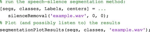
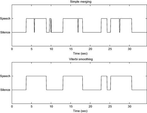
Figure 6.5 Speech-silence segmenter applied on a short-duration signal. The upper figure demonstrates the segmentation results after a naive merging post-processing stage has been performed. The lower figure presents the sequence of labels at the output of the Viterbi-based approach.
6.1.1.4 Example: Fixed-Window Multi-Class Segmentation
This section presents a segmentation example that involves the classes of silence, male speech, female speech, and music. The training data that we need are stored in the model4.mat file. The segmenter employs a multi-class ![]() -NN classifier on a mid-term segment basis. We have created (and stored in a WAVE file) a synthetic audio signal in which all the above classes are present. The ground-truth endpoints of the segments and the respective class labels are stored in a separate mat file for evaluation purposes. We use function segmentationCompareResults() to visualize the results and evaluate them against the ground truth. We also plot the posterior probability estimates for each class and each mid-term window. The complete example is implemented in the demoSegmentation2.m file and is presented below:
-NN classifier on a mid-term segment basis. We have created (and stored in a WAVE file) a synthetic audio signal in which all the above classes are present. The ground-truth endpoints of the segments and the respective class labels are stored in a separate mat file for evaluation purposes. We use function segmentationCompareResults() to visualize the results and evaluate them against the ground truth. We also plot the posterior probability estimates for each class and each mid-term window. The complete example is implemented in the demoSegmentation2.m file and is presented below:

The example calls the segmentationProbSeq() function twice, once for each post-processing method (naive merging and Viterbi-based smoothing). The results are illustrated in Figure 6.6. In this example, the Viterbi-based scheme outperforms the naive merger. More specifically, it can be observed that at the output of the Viterbi-based smoother only a small segment of male speech has been misclassified as silence, whereas, the naive merging scheme has misclassified 2 s of male speech as female speech.

Figure 6.6 Fixed-window segmentation with an embedded ![]() -class classifier (silence, male speech, female speech, and music).
-class classifier (silence, male speech, female speech, and music).
6.1.2 Joint Segmentation-Classification Based on Cost Function Optimization
In this section, audio segmentation is treated as a maximization task, where the solution is obtained by means of dynamic programming [24]. The segmenter seeks the sequence of segments and respective class labels that maximize the product of posterior class probabilities, given the data that form the segments. Note that an increased understanding of this method can be gained if you consult, in parallel, Section 7.3 with respect to the Viterbi-related issues that are also involved in the current section.
To proceed further, some assumptions and definitions must be given. Specifically, it is assumed that each detected segment is at least ![]() frames long, where
frames long, where ![]() is a user-defined parameter. This is a reasonable assumption for the majority of audio types. Furthermore, it is assumed that the duration of a segment cannot exceed
is a user-defined parameter. This is a reasonable assumption for the majority of audio types. Furthermore, it is assumed that the duration of a segment cannot exceed ![]() frames. As will be made clear later in this section, this is a non-restrictive assumption dictated by the dynamic programming nature of the segmenter; any segment longer than
frames. As will be made clear later in this section, this is a non-restrictive assumption dictated by the dynamic programming nature of the segmenter; any segment longer than ![]() will be partitioned in segments shorter than
will be partitioned in segments shorter than ![]() frames.
frames.
Let ![]() be the length of a sequence,
be the length of a sequence, ![]() , of feature vectors, that has been extracted from an audio stream. If
, of feature vectors, that has been extracted from an audio stream. If ![]() are the frame indices that mark the boundaries of the segments, then a sequence of
are the frame indices that mark the boundaries of the segments, then a sequence of ![]() segments can be represented as a sequence of pairs:
segments can be represented as a sequence of pairs:
![]()
where ![]() and
and ![]() . In addition, if
. In addition, if ![]() is the class label of the
is the class label of the ![]() th segment, then
th segment, then ![]() is the posterior probability of the class label
is the posterior probability of the class label ![]() given the feature sequence within the
given the feature sequence within the ![]() th segment. For any given sequence of
th segment. For any given sequence of ![]() segments and corresponding class labels, we can now form the cost function,
segments and corresponding class labels, we can now form the cost function, ![]() as follows:
as follows:
Function ![]() needs to be maximized over all possible
needs to be maximized over all possible ![]() and
and ![]() , under the two assumptions made in the beginning of this section. Therefore, the number of segments,
, under the two assumptions made in the beginning of this section. Therefore, the number of segments, ![]() , is an outcome of the optimization process. Obviously, an exhaustive search is computationally prohibitive, so we resort to a dynamic programming solution. To simplify our presentation, we focus on a speech/music (S/M) scenario, although the method is valid for any number of classes.
, is an outcome of the optimization process. Obviously, an exhaustive search is computationally prohibitive, so we resort to a dynamic programming solution. To simplify our presentation, we focus on a speech/music (S/M) scenario, although the method is valid for any number of classes.
We first construct a grid by placing the feature sequence on the x-axis and the classes on the y-axis (Figure 6.7). A node, ![]() , stands for the fact that a speech segment ends at frame index
, stands for the fact that a speech segment ends at frame index ![]() (a similar interpretation holds for the
(a similar interpretation holds for the ![]() nodes). As a result, a path of
nodes). As a result, a path of ![]() nodes,
nodes, ![]() , corresponds to a possible sequence of segments, where
, corresponds to a possible sequence of segments, where ![]() , and
, and ![]() are the respective class labels. The transition
are the respective class labels. The transition ![]() implies that a segment with class label
implies that a segment with class label ![]() ends at frame
ends at frame ![]() ; and the next segment in the sequence starts at frame
; and the next segment in the sequence starts at frame ![]() , ends at frame
, ends at frame ![]() and has class label
and has class label ![]() . We then associate a cost function,
. We then associate a cost function, ![]() , with the transition
, with the transition ![]() , as follows:
, as follows:
In other words, the cost of the transition is set equal to the posterior probability of the class label, ![]() , given the feature sequence defining the segment
, given the feature sequence defining the segment ![]() .
.
Based on Eqs. (6.1) and (6.2), the cost function, ![]() , becomes:
, becomes:
According to Eq. (6.3), the value of ![]() for a sequence of segments and corresponding class labels can be equivalently computed as the cost of the respective path of nodes in the grid. This means that the optimal segmentation can be treated as a best-path sequence on the grid. The rest of the solution is Viterbi-based processing, the principles of which are further explained in Section 7.3.
for a sequence of segments and corresponding class labels can be equivalently computed as the cost of the respective path of nodes in the grid. This means that the optimal segmentation can be treated as a best-path sequence on the grid. The rest of the solution is Viterbi-based processing, the principles of which are further explained in Section 7.3.
Note that the method requires estimates of the posterior probabilities, ![]() , of the class labels given the candidate segments. In [24], a Bayesian network combiner is used as a posterior probability estimator but this is not a restrictive choice. We can also use a
, of the class labels given the candidate segments. In [24], a Bayesian network combiner is used as a posterior probability estimator but this is not a restrictive choice. We can also use a ![]() -NN scheme that operates on mid-term statistics drawn from the feature sequence of each segment, as has already been demonstrated in previous sections. At the end of this chapter you are asked to implement this dynamic programming-based segmenter as an exercise. You will need to consult Section 7.3 to gain an understanding of those dynamic programming concepts that underlie the operation of the Viterbi algorithm.
-NN scheme that operates on mid-term statistics drawn from the feature sequence of each segment, as has already been demonstrated in previous sections. At the end of this chapter you are asked to implement this dynamic programming-based segmenter as an exercise. You will need to consult Section 7.3 to gain an understanding of those dynamic programming concepts that underlie the operation of the Viterbi algorithm.
6.2 Segmentation Without Classification
Section 6.1 presented segmentation techniques that rely on a trained classifier. However, this is not feasible in every application context. Consider, for example, the problem of speaker clustering (also known as speaker diarization, [64, 68]), where the goal is to partition a speech signal into homogeneous segments with respect to speaker identity. In such problems, there is no prior knowledge regarding the identity of the speakers, so it is not feasible to employ a classifier during the segmentation procedure.
In order to provide a solution, we resort to unsupervised segmentation approaches. The techniques that fall in this category can be further divided into two groups:
• Signal change detection methods: The output simply consists of the endpoints of the detected segments. Information related to the respective labels is not returned by the algorithm.
• Segmentation with clustering: The detected segments are clustered and the resulting clusters are used to assign labels. Speaker diarization solutions fall into this group of methods.
6.2.1 Signal Change Detection
The core idea of signal change detection is to determine when significant changes occur in the content of the audio signal. The detected changes define the boundaries of the resulting segments. Depending on the nature of the signals being studied (e.g. audio from movies, [69], music signals [70], etc.), the detection of endpoints may use a wide range of features and detection techniques.
As an example of this class of methods, we now present an outline of the most important algorithmic steps of an unsupervised detector of signal changes. It is assumed that the input to this method is just the audio signal and that the output consists of a list of pairs of endpoints.
1. Extract a sequence of mid-term feature vectors. This can be achieved with functions stFeatureExtraction() and mtFeatureExtraction() which have already been described.
2. For each pair of successive feature vectors, compute a dissimilarity measure (distance function). As a result, a sequence of distance values is generated.
3. Detect the local maxima of the previous sequence. The locations of these maxima are the endpoints of the detected segments.
The above distance-based approach to audio segmentation is implemented in the segmentationSignalChange() m-file. At the first stage, the function computes mid-term feature statistics for the audio content of a WAVE file:
![]()
The extracted features are then normalized to zero mean and standard deviation equal to one. This linear normalization step prevents features from dominating the computation of the distance measure, i.e. the resulting values are not biased toward features with large values.
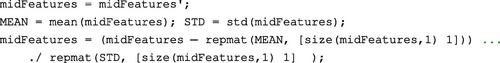
The distance metric is computed using the pdist2() MATLAB function, for each row, i, of the feature matrix:
![]()
Then, we use the findpeaks() MATLAB function of the Signal Processing Toolbox to detect the local maxima of the sequence of distance values:
![]()
As a final step, the peaks whose values are higher than a threshold are preserved. The value of the threshold is equal to the mean value of the sequence of dissimilarities. The use of a threshold filters out local maxima with low values.
We now provide an example of the execution of the segmentationSignalChange() algorithm on an audio signal from a TV program. In order to demonstrate the performance of the function, we have manually annotated the boundaries of segments of the input stream. In addition, we have used function segmentationCompareResults() to visualize the extracted segments and compare them to the results of the manual annotation procedure. To reproduce the example, type the code that is given below (or execute the demoSegmentationSignalChange m-file). The code first loads a .mat file with the true segment boundaries and respective class labels (the latter only serving as auxiliary information in this case).
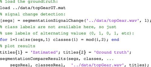
Figure 6.8 presents the results of the segmenter against the manually annotated stream. It can be seen that in most cases the extracted segment limits are in close agreement with the ground truth (label information is ignored in this task, since we are only interested in the segments’ limits and not in their labels).
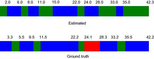
Figure 6.8 Top: Signal change detection results from a TV program. The colors are for illustration purposes and do not correspond to class labels. B: Ground truth. The colors represent different classes but this type of information can be ignored during the evaluation of the performance of the segmenter.
6.2.2 Segmentation with Clustering
The demand for unsupervised segmentation is also raised by certain audio analysis applications that additionally require that the segments are clustered to form groups, so that the segments of each cluster (group) are automatically assigned the same label. Speaker diarization falls in this category of applications; each cluster refers to a different speaker. The output of a diarization system can be seen as a sequence of segments, where each segment has been automatically annotated with the identity (label) of the cluster to which it belongs, e.g., ((![]() ), speaker A),((
), speaker A),((![]() ), speaker B),((
), speaker B),((![]() ), speaker A),((
), speaker A),((![]() ), speaker C), where the
), speaker C), where the ![]() s refer to segment boundaries. In this example, three clusters are formed and one of them, tagged (speaker A), consists of two segments, namely ((
s refer to segment boundaries. In this example, three clusters are formed and one of them, tagged (speaker A), consists of two segments, namely ((![]() ), speaker A) and ((
), speaker A) and ((![]() ), speaker A). In order to understand how speaker diarization and related methods operate, it is firstly important to become familiar with data clustering and related concepts.
), speaker A). In order to understand how speaker diarization and related methods operate, it is firstly important to become familiar with data clustering and related concepts.
6.2.2.1 A Few Words on Data Clustering
So far, we have mainly focused on supervised tasks, where each sample was assigned to a set of predefined audio classes. We are now facing the challenge of dealing with unlabeled data. Our goal is to determine, automatically, the structure of the data. In other words, we are interested in partitioning the dataset of unlabeled samples to a number of subsets, so that the data in each subset are similar to one another and at the same time sufficiently different from the data in other subsets. The procedure that extracts this type of knowledge from a dataset is known as clustering and the resulting subsets as clusters[5, 38, 71–73]. Clustering algorithms require a definition of similarity, so that the generated clusters ‘make sense.’ Due to the fact that similarity can be defined at different levels of abstraction and can address different types of data, it is important to understand that, depending on the application, the adopted similarity measure must serve our needs to optimize the clustering procedure with respect to some appropriately defined criteria. For example, in the case of speaker diarization, a similarity measure needs to be defined among speakers, and the goal of the clustering scheme is to produce a set of clusters that is optimal with respect to the speakers who are present in the audio stream.
A clustering example is shown in Figure 6.9, for an artificially generated dataset consisting of data from four two-dimensional Gaussian distributions. The clustering algorithm was run twice and each time the desired number of clusters was given as input, as it was dictated by the nature of the clustering algorithm that we used (the ![]() -means algorithm). Figure 6.9 b and c present the clustering results for two and four clusters, respectively. Note that, from a visualization perspective, the second clustering seems to provide a better description of the dataset, because the data from each distribution form a separate cluster. However, in practice, it is not always obvious which clustering is a better representative of the dataset and in most cases it is an application-related issue. In a speaker diarization scenario, several different clusterings can be considered to be reasonable depending on the requirements. For example, it makes sense to ask the algorithm to generate two clusters, if we want to split the recording based on the gender of the speaker. A larger number of clusters can be given as input if we are interested in detecting who spoke when and we have obtained prior knowledge about the number of speakers. If the number of clusters is larger than the number of speakers, the resulting clusters may, for instance, end up associated with the emotional state of the speaker(s). In other words, the quality of a clustering can be subjective and depends on the desired outcome of the system under development.
-means algorithm). Figure 6.9 b and c present the clustering results for two and four clusters, respectively. Note that, from a visualization perspective, the second clustering seems to provide a better description of the dataset, because the data from each distribution form a separate cluster. However, in practice, it is not always obvious which clustering is a better representative of the dataset and in most cases it is an application-related issue. In a speaker diarization scenario, several different clusterings can be considered to be reasonable depending on the requirements. For example, it makes sense to ask the algorithm to generate two clusters, if we want to split the recording based on the gender of the speaker. A larger number of clusters can be given as input if we are interested in detecting who spoke when and we have obtained prior knowledge about the number of speakers. If the number of clusters is larger than the number of speakers, the resulting clusters may, for instance, end up associated with the emotional state of the speaker(s). In other words, the quality of a clustering can be subjective and depends on the desired outcome of the system under development.
Figure 6.9 A clustering example in the two-dimensional feature space. The two results correspond to different numbers of clusters (2 and 4). The figures have been generated using the provided demoCluster_general() function.
A well-known and computationally efficient clustering algorithm, which has traditionally been adopted in diverse application fields, is the ![]() -means algorithm [71, 74]. Its goal is to provide the clustering that minimizes a cost-function, which is known to be a NP-hard task [75, 76]. However, despite the complexity of the task, the
-means algorithm [71, 74]. Its goal is to provide the clustering that minimizes a cost-function, which is known to be a NP-hard task [75, 76]. However, despite the complexity of the task, the ![]() -means algorithm can, in general, provide useful suboptimal solutions. The steps of the algorithm are summarized below. It is assumed that the number of clusters,
-means algorithm can, in general, provide useful suboptimal solutions. The steps of the algorithm are summarized below. It is assumed that the number of clusters, ![]() , is given as input:
, is given as input:
1. Select an initial clustering of ![]() clusters. Each cluster is represented by a mean vector, the centroid of its data points.
clusters. Each cluster is represented by a mean vector, the centroid of its data points.
2. Assign each sample of the dataset to the cluster with the nearest centroid. The proximity can be computed with the Euclidean distance function.
3. Update the centroid of each cluster using all the samples that were assigned to the cluster during the previous step.
4. Repeat from step 2 until it is observed that the clustering remains the same in two successive iterations of the algorithm.
The operation of the ![]() -means algorithm is affected by the number of clusters at the input, the initialization scheme (initial clustering), and the choice of distance metric. The estimation of the number of classes is not a trivial issue. A possibility is to run the
-means algorithm is affected by the number of clusters at the input, the initialization scheme (initial clustering), and the choice of distance metric. The estimation of the number of classes is not a trivial issue. A possibility is to run the ![]() -means algorithm for a range of values of the
-means algorithm for a range of values of the ![]() parameter and select the ‘best’ solution after evaluating each clustering against a quality criterion [77, 78]. The task of estimating the number of clusters is presented in more detail in Section 6.2.2.1.1. The initialization of the algorithm is also of crucial importance for its convergence to an acceptable solution. A well-known technique is to initialize the algorithm randomly a number of times and select as the winner the most frequently appearing clustering or the clustering that corresponds to the lowest value of the cost function.
parameter and select the ‘best’ solution after evaluating each clustering against a quality criterion [77, 78]. The task of estimating the number of clusters is presented in more detail in Section 6.2.2.1.1. The initialization of the algorithm is also of crucial importance for its convergence to an acceptable solution. A well-known technique is to initialize the algorithm randomly a number of times and select as the winner the most frequently appearing clustering or the clustering that corresponds to the lowest value of the cost function.
The ![]() -means algorithm is a typical centroid-based technique because each cluster is represented by its centroid (note that centroids do not necessarily coincide with points of the dataset). Another important category of clustering methods consists of the so-called hierarchical clustering algorithms. The goal of these algorithms is to produce a hierarchy of clusters given the points of a dataset. The extracted hierarchy is presented as a tree-like structure [72]. The two dominant trends in the field of hierarchical clustering are the agglomerative and divisive techniques:
-means algorithm is a typical centroid-based technique because each cluster is represented by its centroid (note that centroids do not necessarily coincide with points of the dataset). Another important category of clustering methods consists of the so-called hierarchical clustering algorithms. The goal of these algorithms is to produce a hierarchy of clusters given the points of a dataset. The extracted hierarchy is presented as a tree-like structure [72]. The two dominant trends in the field of hierarchical clustering are the agglomerative and divisive techniques:
• Agglomerative methods. In the beginning of the algorithm, the number of clusters is equal to the number of samples, i.e. each cluster contains only one sample. At each iteration, the two most similar clusters are merged and the procedure is repeated until a termination criterion is satisfied [79]. The agglomerative algorithms follow a bottom-up approach because the number of clusters is reduced by one at the end of each iteration.
• Divisive methods. These algorithms adopt a top-down approach. They start with a root cluster that contains the entire dataset and perform an iterative splitting operation based on an adopted criterion [80, 81].
In recent years, we have also witnessed the increasing popularity of spectral clustering techniques [73, 82–84]. The key idea behind spectral clustering is that the dataset is first represented as a weighted graph, where the vertices correspond to data points and the edges capture similarities between data points. Clustering is then achieved by cutting the graph in to disconnected components so that an optimization criterion is fulfilled. Another modern approach to data clustering is provided by the Non-Negative Matrix Factorization (NMF) methodology, which approaches the problem of clustering from the perspective of concept factorization [73, 85–88]. NMF techniques treat each data point as a linear combination of all cluster centers. Applications of NMF include sound source separation [89] and document clustering [85].
6.2.2.1.1 Estimating the Number of Clusters
Several solutions have been proposed in the literature for the estimation of the number of clusters in a dataset [77, 90–92]. A popular approach is to execute the ![]() -means algorithm for a range of values of parameter
-means algorithm for a range of values of parameter ![]() and select the optimal clustering, based on a selected criterion, like the ‘gap statistic’ [77]. In this section, we have adopted the Silhouette method proposed in [92]. This is a simple method that measures how ‘tightly’ the data are grouped in each cluster, using a distance metric. The Silhouette method is implemented in the silhouette() function of the Statistics Toolbox. Figure 6.10 presents a clustering example where the Silhouette method was used to estimate the number of clusters. It can be observed that the Silhouette measure is maximized when the number of clusters is 4 and this is the adopted solution in this case. Note that some clustering approaches, e.g. the hierarchical clustering methods, may embed the estimation of the number of clusters in the clustering procedure itself.
and select the optimal clustering, based on a selected criterion, like the ‘gap statistic’ [77]. In this section, we have adopted the Silhouette method proposed in [92]. This is a simple method that measures how ‘tightly’ the data are grouped in each cluster, using a distance metric. The Silhouette method is implemented in the silhouette() function of the Statistics Toolbox. Figure 6.10 presents a clustering example where the Silhouette method was used to estimate the number of clusters. It can be observed that the Silhouette measure is maximized when the number of clusters is 4 and this is the adopted solution in this case. Note that some clustering approaches, e.g. the hierarchical clustering methods, may embed the estimation of the number of clusters in the clustering procedure itself.
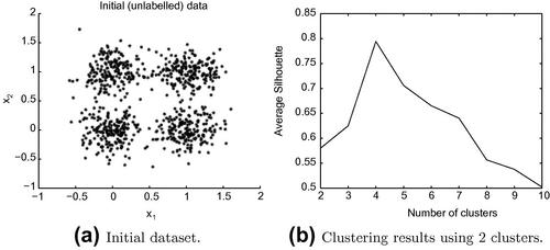
Figure 6.10 Silhouette example: the average Silhouette measure is maximized when the number of clusters is 4. This example was generated using the demoCluster_generalSil() function that can be found in the software library that accompanies this book.
6.2.2.1.2 Data Clustering Functionality in MATLAB
MATLAB includes several functions that perform data clustering. In this section we provide a brief description of the ![]() -Means algorithm and the agglomerative clustering technique.
-Means algorithm and the agglomerative clustering technique.
The ![]() -Means algorithm has been implemented in the kmeans() function of the Statistics Toolbox. The function takes as input a data matrix with one feature vector per row along with the desired number of clusters. It returns a vector of cluster labels for the data points, as well as the centroids of the clusters in a separate matrix. If the user demands a deeper understanding of the operation of the algorithm, more output arguments are possible, e.g. the within-cluster sums of point-to-centroid distances.
-Means algorithm has been implemented in the kmeans() function of the Statistics Toolbox. The function takes as input a data matrix with one feature vector per row along with the desired number of clusters. It returns a vector of cluster labels for the data points, as well as the centroids of the clusters in a separate matrix. If the user demands a deeper understanding of the operation of the algorithm, more output arguments are possible, e.g. the within-cluster sums of point-to-centroid distances.
The Statistics Toolbox also supports the agglomerative (hierarchical) clustering method. To use the respective functionality, take the following steps:
1. Use the pdist() MATLAB function to compute the similarity (or dissimilarity) between every pair of samples of the dataset.
2. Form a hierarchical tree structure using the linkage() function, which provides the agglomerative functionality. The resulting structure is encoded in a specialized matrix format.
3. Use the cluster() function to transform the output of the linkage() function to a set of clusters based on a thresholding criterion.
The above three-step agglomerative procedure can also be executed in a single step using the MATLAB function clusterdata(). We have provided a stepwise description so that the reader becomes familiar with the key mechanism on which agglomerative clustering operates.
6.2.2.1.3 Semi-Supervised Clustering
In many clustering applications, although the dataset is unlabeled, there exists auxiliary information that can be exploited by the clustering algorithm to yield more meaningful results. Such methods are usually referred to as semi-supervised clustering techniques [71, 93, 94].
A popular approach to semi-supervised clustering is to make use of pair-wise constraints. For example, a ‘must-link’ constraint can specify that two samples from the dataset must belong to the same cluster. This type of constraint has been used in the field of speaker clustering. The work in [64] proposes a semi-supervised approach that groups speech segments to clusters (speakers) by making use of the fact that two successive segments have a high probability of belonging to the same speaker. This auxiliary information has been proven to boost the performance of the clustering scheme.
6.2.2.2 A Speaker Diarization Example
In this section, we provide the description and respective MATLAB code of a simple speaker diarization system. Remember that speaker diarization is the task of automatically partitioning an audio stream into homogeneous segments with respect to speaker identity [64, 68, 95]. The input of a speaker diarization (SD) method is a speech signal, without any accompanying supervised knowledge concerning the speakers who are involved. The goal of a SD system is to:
• Estimate the number of speakers.
• Estimate the boundaries of speaker-homogeneous segments.
• Map each segment to a speaker ID.
For the sake of simplicity, we will only describe the main speaker diarization functionality, assuming that the number of speakers is provided by the user. Of course, generally in the general case, the number of speakers is unknown and has to be estimated using a suitable method like the one in Section 6.2.2.1.1. A schematic description of our diarization method is shown in Figure 6.11. The respective source code can be found in the speakerDiarization() function of the software library that accompanies this book. The method involves the following steps:
1. Computes feature statistics on a fixed-length segment basis using the featureExtractionFile() function already used several times in this book. The result of this procedure is a sequence of vectors of feature statistics and a sequence of time stamps (in seconds), which refer to the time equivalent of the centers of the mid-term segments.
2. The feature statistics, which were extracted in the first step, are linearly normalized to zero mean and unity standard deviation. The normalization step increases the robustness of the clustering procedure.
3. The (normalized) feature statistics are used by the ![]() -Means clustering algorithm, which assigns a cluster identity to each mid-term segment. Apart from the segment labels, the clustering algorithm also returns the distances of the feature vectors (representing the segments) from all the centroids. This is the 4th output argument of the kmeans() function of the Statistics Toolbox. The computed distances form a
-Means clustering algorithm, which assigns a cluster identity to each mid-term segment. Apart from the segment labels, the clustering algorithm also returns the distances of the feature vectors (representing the segments) from all the centroids. This is the 4th output argument of the kmeans() function of the Statistics Toolbox. The computed distances form a ![]() matrix,
matrix, ![]() , where
, where ![]() is the number of clusters and
is the number of clusters and ![]() is the number of segments.
is the number of segments.
4. The distance matrix is used to provide a crude approximation of the probability that a segment belongs to a cluster. This is achieved by computing the quantity ![]() for each element of
for each element of ![]() and then by normalizing the resulting values column-wise. The result of this step is a
and then by normalizing the resulting values column-wise. The result of this step is a ![]() matrix
matrix ![]() , whose elements,
, whose elements, ![]() , represent the estimated probability that sample (segment)
, represent the estimated probability that sample (segment) ![]() belongs to cluster
belongs to cluster ![]() . Each row of this matrix is subsequently smoothed using a simple moving average technique.
. Each row of this matrix is subsequently smoothed using a simple moving average technique.
5. The probabilistic estimates are then given as input to the segmentationProbSeq() MATLAB function (already described in Section 6.1.1.1), which produces the final list of segments and respective cluster labels.

Figure 6.11 Block diagram of the speaker diarization method implemented in speakerDiarization(). ![]() is the matrix of feature statistics of all segments and
is the matrix of feature statistics of all segments and ![]() is its normalized version.
is its normalized version. ![]() is the distance matrix, which is returned by the
is the distance matrix, which is returned by the ![]() -means algorithm.
-means algorithm. ![]() is the matrix of probability estimates, which is used in the final segmentation stage to generate the detected segment boundaries and corresponding cluster labels.
is the matrix of probability estimates, which is used in the final segmentation stage to generate the detected segment boundaries and corresponding cluster labels.
The following code demonstrates how to call the speakerDiarization() function and plot its results using the segmentationPlotResults() function:

Figure 6.12 presents the results of the application of the speaker diarization method. Note that the speakerDiarization() function implements a typical clustering-based audio segmentation technique. The reason that we have focused on speaker diarization is that it is a well-defined task with meaningful results. The same function can be used in any clustering-based audio segmentation application. The reader is encouraged to test the function on other types of audio signals, e.g. on a music track, and provide an interpretation of the resulting segments. In general, music segmentation is a very different task from speaker diarization, requiring different features and techniques. More on selected music analysis applications are presented in Chapter 8.

Figure 6.12 Visualization of the speaker diarization results obtained by the speakerDiarization() function (visualization is obtained by calling the segmentationPlotResults() function). Different colors represent different speaker labels. The lower part of the figure represents the waveform of an audio segment, which was selected by a user.
6.3 Exercises
1. (D3) Follow the instructions given below in order to create a MATLAB function that implements a speech-silence segmenter that employs a binary classifier:
• Load the model4.mat file, keep the data that refer to the classes of speech and silence, and discard the rest. Create a classification setup for the speech vs silence task and store the data in the modelSpeechVsSilence.mat file.
• Reuse the code that was presented in this chapter to design a fixed-window segmenter that adopts a ![]() -NN classifier.
-NN classifier.
• Record a speech signal to demonstrate your implementation and compare the results with those obtained by the silenceRemoval() function of Section 6.1.1.3.
2. (D3) Section 6.1.1.1 presented a segmenter that was based on a ![]() NN classifier of fixed-length windows, using the speech-music dataset of the modelSM.mat file. In this exercise you are asked to:
NN classifier of fixed-length windows, using the speech-music dataset of the modelSM.mat file. In this exercise you are asked to:
• Annotate manually the speech_music_sample.wav file from the data folder of the companion material. You will need to create a mat-file (speech_music_sampleGT.mat) that contains annotations of the same format as the output of the segmentationProbSeq function, i.e.: (a) a 2-column matrix of segment boundaries, and (b) an array of class labels (0 for speech and 1 for music).
• Run functions mtFileClassification() and segmentationProbSeq() to segment the speech_music_sample.wav file using the modelSM.mat file for the classification task. This needs to be done for both methods supported by segmentationProbSeq().
• Use function segmentationCompareResults() to compare the results of both post-processing techniques with the ground truth that you have created.
Hint: In Section 6.1.1.4 we demonstrated the same task for a 4-class scenario. Here, you only need to create ground truth data for a WAVE file and then go through the steps of Section 6.1.1.4, using the modelSM.mat file.
3. (D5) Implement a variant of a region growing technique that splits an audio stream into speech and music parts [24]. The main idea is that each segment can be the result of a segment (region) growing technique, where one starts from small regions and keeps expanding them as long as a predefined threshold-based criterion is fulfilled. To this end, implement the following steps:
(a) Extract the short-term feature of spectral entropy from the audio recording (see Chapter 4). Alternatively, you can use the entropy of the chroma vector.
(b) Select a number of frames as candidates (seeds) for region expansion. The candidates should preferably be equidistant, e.g. one candidate every 2 s (user-defined parameter).
(c) Starting from the seeds, segments grow to both directions and keep expanding as long as the standard deviation of the feature values in each region remains below a predefined threshold. Note that a feature value can only belong to a single region. Therefore, a region ceases to grow if both its neighboring feature values already belong to other regions. At this end of this processing stage, the resulting segments contain music and all the rest is speech.
(d) Post-processing: adjacent segments are merged and short (isolated) segments are ignored. All segments that have survived are labeled as music, because the algorithmic parameters are tuned toward the music part of the signal.
Your function must receive as input a WAVE file, the type of feature, the distance between successive seeds (in seconds), and the threshold value for the region growing step. The segmentation results must conform with the output format that has been adopted in the chapter. Experiment with different threshold values and comment on the results. Compare the performance of your implementation with a fixed-window segmenter that uses a binary classifier for the task of speech vs music.
4. (D5) Implement the Viteri-based solution of Eq. (6.3). Use a ![]() -NN estimator for the posterior probabilities. Your function must take as input the path to a WAVE file, the short-term features to be extracted, the segment duration constraints, and the mid-term statistics that will be used during the estimation of the posterior probabilities. You will need to consult Chapter 7 in order to gain an understanding of the dynamic programming concepts that underlie the operation of the Viterbi algorithm. On a 4-class problem, compare the results of this method with the performance of a fixed-window technique.
-NN estimator for the posterior probabilities. Your function must take as input the path to a WAVE file, the short-term features to be extracted, the segment duration constraints, and the mid-term statistics that will be used during the estimation of the posterior probabilities. You will need to consult Chapter 7 in order to gain an understanding of the dynamic programming concepts that underlie the operation of the Viterbi algorithm. On a 4-class problem, compare the results of this method with the performance of a fixed-window technique.
5. (D1) The core technique in the speakerDiarization() function is a generic clustering-based audio segmenter. Therefore, it makes sense to try and use it with non-speech signals. Experiment with the speakerDiarization() and segmentationPlotResults() functions on music tracks and assign meaning (if possible) to the clustering results.
6. (D3) Create a Matlab function that extends the functionality of the speakerDiarization() method by computing a confidence measure for each detected segment. Such a measure can be quite useful in various applications. For instance, one could use it to filter out segments that correspond to low confidence values, so that the algorithm outputs only those segments for which confidence is sufficiently high. Furthermore, the confidence measure can be adopted by fusion techniques (e.g. jointly with visual-oriented cues). Hint: Compute the average estimated probability (using the Ps matrix in the speakerDiarization() function) at each segment over all fixed-sized windows contained in that segment.
7. (D5) Assume that, in a speaker diarization context, the number of speakers has not been provided by the user. Extend the functionality of the speakerDiarization() function by adding an estimator for the number of clusters (speakers). To achieve this goal, use the Silhouette method that was explained in Section 6.2.2.1.1. The new function must receive a single input argument, i.e. the path to the audio file to analyze.
8. (D4) The speakerDiarization() function estimates, for each segment, the probability that the segment belongs to each cluster. However, this is achieved in a rather simple manner (using the inverse distance from each cluster centroid). Modify the speakerDiarization() function so that the probability estimate is computed by means of a more sophisticated technique. This can be obviously achieved in many ways and the reader can choose any valid probability estimation method. Here, we propose that you use a ![]() -NN classifier that exploits the centroids of the clusters at the output of the
-NN classifier that exploits the centroids of the clusters at the output of the ![]() -means algorithm in order to estimate the probability that each segment belongs to a cluster.
-means algorithm in order to estimate the probability that each segment belongs to a cluster.
9. (D4) The speakerDiarization() function assumes that the input signal contains only speech. However, if long intervals of silence/background noise are also present, reduced performance may be observed. Combine speakerDiarization() and silenceRemoval() to filter out areas of silence from the input signal before the clustering scheme is employed.
10. (D3) The signal change detection approach in Section 6.2.1 extracts segments of homogeneous content without making use of any type of supervised knowledge. In several audio applications, such a functionality can be used as a first step in a segmentation - classification system. In this exercise, combine:
• Function segmentationSignalChange() to extract homogeneous audio segments from an audio stream.
• The feature extraction and classification process (see Chapter 5) to classify (k-NN) each extracted segment as music or speech (use modelSM.mat).
Hint: The feature extraction and classification processes must be applied on each segment (extracted by the signal change detection step), using the following sequence of operations: (a) short-term feature extraction, (b) mid-term statistics generation, (c) long-term averaging of the statistics for the whole segment, and (d) application of the classifier. The same sequence of steps was followed in the fileClassification() function.