Audio Alignment and Temporal Modeling

This chapter presents several methods that take into account the temporal evolution of the audio phenomena. In other words, we are no longer interested in computing mid-term feature statistics or long-term averages from the audio signals. On the contrary, our main concern is to preserve the short-term nature of the feature sequences in order to (a) devise techniques that are capable of aligning two feature sequences, and (b) build parametric, temporal representations of the audio signals by means of the Hidden Markov modeling methodology. The two goals are complementary in the sense that the former involves non-parametric approaches, whereas the latter aims at deriving parametric stochastic representations of the time-varying nature of the signals. The choice of method depends on the application and the availability of training data. Sometimes non-parametric techniques are the only option, as is, for example, the case with query-by-example scenarios where the user provides an audio example that needs to be detected in a corpus of audio recordings. On the other hand, if sufficient training data are available, it might be preferable to build parametric models, as has traditionally been the case in the speech recognition literature. The chapter starts with sequence alignment techniques and proceeds with a description of the Hidden Markov models (HMMs) and related concepts. We have found it necessary to provide lengthier theoretic descriptions in this chapter. However, care has been taken, so that the presentation is given from an engineering perspective, in order to facilitate the realization of practical solutions.

7.1 Audio Sequence Alignment

In the field of content-based audio retrieval, it is often useful to detect occurrences of an audio pattern in an audio stream, match audio data of varying lengths to a set of predefined templates, compare audio recordings to identify similar parts, and so on. The related terminology has its origins in speech processing literature, where similar problems have been intensively studied over past decades. For example, in an analogy of the word spotting problem in the speech recognition context, we can define the audio spotting or audio tracking task, where the goal is to detect occurrences of an audio example in a corpus of audio data. The audio example can be a digital audio effect that we need to track in the audio stream of a movie or a specific sound of a mammal that is likely to be repeated in a corpus of underwater recordings of very long duration. An endless list of similar examples can be compiled for a diversity of applications, ranging from intrusion detection systems to query-by-humming services. It is important to realize that we are interested in providing non-parametric solutions, i.e. we assume that we have not previously built parametric models that describe the problem at hand, based on prior knowledge.

An important requirement in such application scenarios is the ability to align feature sequences. Although in the literature the term sequence alignment refers to a broad class of problems, we start our discussion with the well-known template matching task, a direct application of which, can be encountered in the design of classifiers, when each class can be represented by one or more reference patterns (prototypes). The key idea behind template matching is that we can quantify how similar (dissimilar) two feature sequences are, even when they are not of equal length. For example, if you record your own voice repeating the word ‘library’ ten times with sufficiently long periods of silence between successive utterances and examine the resulting signals, you will observe that no two words are alike at the signal level. Some phonemes will be of shorter duration, whereas others will last longer, even if the differences are in the order of a few milliseconds. Furthermore, the same phoneme can be louder in some utterances. Yet, all signals are easily perceived by a human as the word ‘library’ and, in addition, if a different word is uttered, we will immediately percieve the difference.

7.1.1 Dynamic Time Warping

In order to deal with the alignment task from an algorithmic perspective, we understand that we need algorithms that are capable of quantifying similarity (dissimilarity) in an optimal way, by taking into account the fact that parts of one sequence may need to be locally stretched or compressed, so that the optimal alignment is achieved. The operations of stretching and compressing audio parts are collectively known as time warping. Due to the fact that time warping is determined dynamically during the joint inspection of two feature sequences, the term Dynamic Time Warping (DTW) is often used to denote the alignment of two feature sequences that represent audio signals.

To proceed further, certain definitions must first be given. Let and , be the two feature sequences to be aligned. In general, and and are -dimensional feature vectors. Furthermore, let be a dissimilarity function, e.g. the Euclidean distance function, which is defined as

(7.1)

The DTW algorithms start with the construction of a cost grid, . Assuming that sequences and X are placed on the horizontal and vertical axis, respectively, the coordinates of node are the th element (feature vector) of X and the th element of R. Subsequently, a dynamic programming algorithm is employed. The algorithm starts from node (1,1) and the nodes of the grid are visited row-wise from left to right (an equivalent column-wise visiting scheme can also be adopted). At each node, we compute the accumulated cost to reach the node. At the end of this processing stage, the cost at node represents the total matching cost between the two feature sequences. A zero cost indicates a perfect match. The higher the matching cost, the more dissimilar (less similar) the two sequences.

Obviously, there are several open questions: which are the nodes from which a node, , can be reached? What is the cost of a transition from one node to another? Why is this procedure capable of generating the optimal matching cost? To answer such questions, we now provide a step-by-step description of two popular DTW schemes, which are based on the so-called Sakoe-Chiba [96] and Itakura [97] local path constraints.

7.1.1.1 The Sakoe-Chiba Local Path Constraints

Initialization: We start with node (1,1) and set . Due to the fact that node (1,1) is the first node that we visit, we define its predecessor as the fictitious node (0,0). We are using a separate matrix, , to store the (best) predecessor of each node. In this case, .

Iteration: We adopt a row-wise visiting scheme (from left to right at each row) and compute the cost, , to reach node , as follows:

(7.2)

Equation (7.2) defines the local path constraints of the DTW scheme. Specifically, it defines that the allowable predecessors of node are the nodes: (diagonal transition); (vertical transition); and (horizontal transition). In addition, it defines that the cost of the transition from a predecessor to node is equal to the local cost (dissimilarity) between and . The node that minimizes Eq. (7.2) is the best predecessor of node and its coordinates are stored in the matrix. The value stands for the optimal (lowest) cost to reach node , i.e. the more efficient way to reach the node, given the local path constraints. This is guaranteed by Bellman’s optimality principle [98], which states that the optimal path to reach node from (1,1) is also optimal for each one of the nodes that constitute the path.

Termination: After the accumulated cost has been computed for all nodes, we focus on node . The cost to reach this node is the overall matching cost between the two feature sequences. To extract the respective optimal path, we perform a backtracking procedure: starting from node , we visit the chain of predecessors until we reach the fictitious node (0,0), which is the predecessor of node (1,1). The extracted chain of nodes is known as the best (optimal) path of nodes.

Horizontal and vertical transitions in the best path imply that certain time warping was necessary in order to align the two sequences; the longer the horizontal and vertical transitions, the more intense the time warping phenomenon. The Sakoe-Chiba constraints permit arbitrarily long sequences of horizontal or vertical transitions to take place, which implies that they do not impose any time warping limits. This is not always a desirable behavior, hence the need for other types of local constraints, like the Itakura constraints, which are described next.

We provide an implementation of the Sakoe-Chiba DTW scheme in the dynamicTimeWarpingSakoeChiba() function. To call this function, type:

The first two input arguments are the -dimensional feature sequences to be aligned. Sequence is placed on the vertical axis of the grid. The third argument is set to ‘1’ if we want to divide the resulting matching cost (first output argument) by the length (number of nodes) of the best path. This type of normalization is desirable when the DTW scheme is embedded in a classifier that matches unknown patterns against a set of prototypes, because the normalized cost is an arithmetic average that is independent of the length of the sequences that are being matched. The second output argument is the sequence of nodes (pairs of indices) of the optimal alignment path.

7.1.1.2 The Itakura Local Path Constraints

In several audio alignment tasks it is undesirable to permit arbitrarily long sequences of horizontal and vertical transitions, because we expect that two instances of an audio pattern cannot be radically different. It is possible to account for this requirement, if we replace the Sakoe-Chiba scheme with a different set of local constraints. A popular choice are the Itakura local path constraints [97], which are defined as:

(7.3)

First of all, it can be easily observed that vertical transitions are not allowed at all. Secondly, it is possible to omit feature vectors from the sequence that has been placed on the vertical axis (one feature vector at a time), due to the fact that node is an allowable predecessor. A third important remark is that two successive horizontal transitions are not allowed due to the constraint that demands . These properties ensure that time warping cannot be an arbitrarily intense phenomenon. An implication of the Itakura constraints is that . Furthermore, the Itakura constraints are asymmetric because, in the general case, if the sequences change axes, the resulting matching cost will be different (on the contrary, the Sakoe-Chiba constraints are symmetric).

The Itakura algorithm is initialized like the Sakoe-Chiba scheme and Eq. (7.3) is repeated for every node. In the end, node has accumulated the matching cost of the two sequences. The backtracking stage extracts the optimal sequence of nodes, assuming again that the best predecessor of each node has been stored in a separate matrix.

The software library that accompanies this book contains an implementation of the Itakura algorithm in the dynamicTimeWarpingItakura() function. To call this function, type:

For the sake of uniformity, we have preserved the input and output formats of the dynamicTimeWarpingSakoeChiba() function. Both functions have adopted the Euclidean distance as a dissimilarity measure.

7.1.1.3 The Smith-Waterman Algorithm

The Smith-Waterman (S-W) algorithm was originally introduced in the context of molecular sequence analysis [99]. It is a sequence alignment algorithm that can be used to discover similar patterns of data in sequences consisting of symbols drawn from a discrete alphabet.

An important characteristic of the S-W algorithm is that it employs a similarity function that generates a positive value to denote similarity between two symbols and a negative value for the case of dissimilarity. In addition, it introduces a gap penalty to reduce the accumulated similarity score of two symbol sequences when a part of one sequence is missing from the other. The algorithm is based on a standard dynamic programming technique to reveal the two subsequences that correspond to the optimal alignment. In the field of music information retrieval, the S-W algorithm has been used to provide working solutions for the tasks of cover song identification [100], query-by-humming [101], and melodic similarity [102]. In the more general context of audio alignment, variants of the algorithm that operate on a continuous feature space have been presented in [103,104].

In order to proceed with the description of the original S-W algorithm, let and be two symbol sequences, for which and , are the th and th symbol, respectively. We first need to define a function, , that takes as input two discrete symbols, and returns a measure of their similarity. The similarity function, , is defined as

(7.4)

At the next stage, we construct a similarity grid, . We assume that the rows and columns of the grid are indexed and , respectively. Each node of the grid is represented as a pair of coordinates, . The basic idea of the algorithm is that each node accumulates a similarity score by examining a set of nodes known as predecessors. After the accumulated score has been computed for all the nodes of the grid, the node with the highest score wins and a backtracking procedure reveals the two symbol subsequences that have contributed to this maximum score.

Initialization: The first row and column of the grid are initialized with zeros:

Iteration: For each node, , of the grid, we compute the accumulated similarity cost:

(7.5)

A closer inspection of Eq. (7.5) reveals that node can be reached from the following predecessors:

If, on the other hand, the accumulated score is positive, the best predecessor, , of is the node that maximizes ,

(7.6)

Equations (7.5) and (7.6) are repeated for all nodes of the grid, starting from node (1,1) and moving from left to right (increasing index ) and from the bottom to the top of the grid (increasing index ). Concerning the first row and first column of the grid, the predecessor is always set to the fictitious node (0,0). All predecessors, , are stored in a separate matrix to enable the final processing stage (the backtracking operation).

Backtracking: After has been computed for all nodes, we select the node that corresponds to the maximum score and follow the chain of predecessors until we encounter a (0,0) node (the algorithm ensures that a (0,0) node will definitely be encountered). The resulting chain of nodes is the best (optimal alignment) path. The coordinates of the nodes of the best path reveal the subsequences of and , which have been optimally aligned, and indicate which symbol deletions have taken place. The backtracking procedure can be repeated to generate the second best alignment and so on. Care has to be taken so that each new backtracking operation ignores the nodes that have already participated in the preceding optimal paths.

We have implemented the standard S-W algorithm in the smithWaterman() function. To reproduce the example in the original paper ([99]), type:

The first two arguments are molecular sequences and the third argument controls the gap penalty. The fourth argument is set to ‘1’ because we want to have the output of the alignment procedure printed on the screen. If the last argument is set to ‘1’, then a figure with the best path is also plotted. The printout of the function call is:

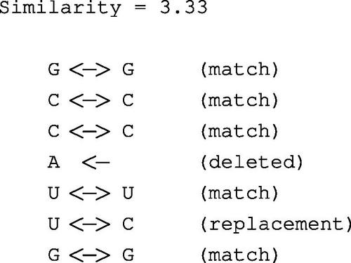
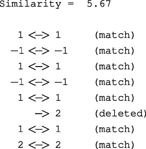
It can be seen that has been aligned with . The second subsequence is one symbol shorter, hence the deletion of symbol . The deletion reduces the accumulated similarity score by . Furthermore, the mapping of to is equivalent to a symbol replacement that reduces the similarity score by . This is why the alignment score is equal to . Instead of character strings, we can also use the smithWaterman() function to align any type of sequences consisting of discrete symbols. The next example uses integers. Type:

In this case, the output on the screen is:

7.2 Hidden Markov Modeling

A Hidden Markov Model (HMM) is a stochastic automaton that undergoes distinct transitions among states based on a set of probabilities. When the HMM arrives at a state, it emits an observation, which, in the general case, can be a multidimensional feature vector of discrete or continuous elements. The emission of observations is also governed by probabilistic rules.

During the design of an HMM it is of crucial importance to decide on the number of states and assign a meaningful stochastic interpretation to each state, so that the nature of the problem is reflected successfully on the structure of the HMM. These are not trivial issues in any sense and usually require a careful study of the stochastic nature of the phenomenon for which the HMM will be designed. For example, a phoneme in a speech recognition task can be modeled with a 3-state HMM, because, from a statistical perspective, the phoneme consists of three different parts (segments) and this is also reflected in the properties of most short-term feature sequences that can be extracted from the phoneme (e.g. the sequence of MFCCs). From a simplified point of view, the three parts refer to the beginning, steady state, and attenuation of the phoneme. As another example, in a speech/music/silence segmentation scenario, it can be useful to assign a class label to each state, leading to a 3-state HMM. As a general remark, the number of states is implicitly dictated by the interpretation of the most important stationarity changes in the signals of the problem at hand.

Another important issue has to do with the selection of the most appropriate features for the signals under study. For example, in speech recognition, it has been customary to use vectors of MFCCs as features and this has also turned out to be a more general trend in the field of audio processing. In the general case, the selected features should be able to reflect the temporal evolution of the signal on a short-term basis, without providing excessive detail. The designer of the HMM must be familiar with various audio features (see also Chapter 4) and needs to be able to experiment with their combinations. Usually, the resulting feature vectors are multidimensional and consist of continuous features. However, in order to provide a gentle introduction to the theory of HMMs, we focus on the case of discrete observations.

7.2.1 Definitions

Let be the set of HMM states and the discrete symbols of the alphabet of observations. The following three matrices represent the HMM, namely:

7.2.2 An Example

Consider a 3-state HMM that is capable of emitting two discrete symbols. The HMM is represented by the following matrices:

It can be observed that the HMM always starts at the first state and that matrix is upper triangular. The latter implies that we are dealing with a left-to-right model because backward transitions do not exist, or, equivalently, a transition from a state always ends at a state with a higher index. This type of HMM has been very popular in the speech recognition field because it fits well with the temporal evolution of phonemes, the building blocks of speech utterances.

Now assume that we ask the following question: what is the probability, , that the sequence of states emits the sequence of symbols ? The answer is based on computing the joint probability of the following events:

7.2.3 Some Useful Questions

Given an HMM, , it is important to be able to answer the following questions, which are encountered in almost every application involving HMMs:

After the HMM has been trained, it can be used both as a recognition machine and a generator of observation sequences, depending on the application context. For example, in a classification problem with four classes, we can train one HMM per class. When an unknown feature sequence is to be classified, it is assigned to the class which is represented by the HMM that has produced the highest recognition (or Viterbi) score. HMMs can be used for numerous other tasks, e.g. for audio tracking and segmentation purposes. It would not be an exaggeration to claim that HMM methodology is the driving technology in several machine learning fields, with speech recognition being an outstanding example.

7.3 The Viterbi Algorithm

The goal of the Viterbi algorithm is to discover the optimal sequence of states given an HMM and a sequence of observations. Here, the term optimal is defined from a probabilistic perspective. In other words, the Viterbi algorithm seeks the sequence of HMM states that maximizes the joint probability of observations given the HMM.

The computational complexity of an exhaustive solution to the task is prohibitively high even for small-sized HMMs and short sequences of observations. For example, if a sequence is 30 observations long and an HMM consists of 5 states, the number of all possible state sequences is . It is, therefore, not a surprise that the algorithm resorts to dynamic programming principles to achieve its goal.

More specifically, it creates a cost grid (trellis diagram) by placing the states, of the HMM on the vertical axis and the sequence of observations, , on the horizontal axis. Each node, , accumulates a probabilistic score, , which is interpreted as the probability to reach state , via an optimal sequence of states, after emitting the first observations. The Viterbi algorithm computes the probability for every node of the trellis diagram, starting from the first column (). The maximum value at the last column is, therefore, the probability to emit the complete sequence of observations via an optimal sequence of states, which is subsequently extracted by means of a standard backtracking operation. We now provide a description of the steps of the Viterbi algorithm in the case of discrete observations. Remember that is the vector of initial state probabilities, is the state transition matrix, and is the matrix of observation probabilities (Section 7.2).

Initialization: Assign values to the nodes of the first column of the grid:

It has been assumed that each symbol of the discrete alphabet has been given a positive identity. As a result, the feature sequence is actually a sequence of symbol identities and stands for the probability that the th state emits the symbol with identity .

Iteration: For the th column, , compute the probability :

(7.7)

An interesting observation is that the computation of only takes into account the previous column of the grid (). This is also known as the first-order Markovian property. The equation examines each node of the previous column as a potential predecessor of the node . To this end, , is multiplied with the product , which is interpreted as the joint probability of the transition and the emission of symbol from state . In the end, the winner is the transition that yields the maximum probabilistic score. Bellman’s optimality principle [98] ensures that the resulting value, , will represent the score of the optimal sequence of states that has ended with state and has emitted the subsequence of observations until (including) the th time instant. To enable backtracking, the coordinates of the best predecessor of node are stored in a separate matrix, , so that:

Termination: Detect the maximum value at the last column of the grid. This value is also known as the Viterbi score of the HMM for the given sequence of observations. The node that contains the Viterbi score serves to start a backtracking procedure that visits each column in reverse order until the first column is reached. The resulting chain of nodes reveals the best-state sequence (best-path).

We have implemented the Viterbi algorithm for discrete observations in the scaledViterbiDisObs() function, which is based on a ‘scaling’ technique that deals with arithmetic stability issues due to the repeated multiplication of probabilities. The scaling method is based on the fact that if logarithms are used in Eq. (7.7), the products will be replaced by summations without affecting monotonicity. The scaled version of Eq. (7.7) is

(7.8)

To call the scaledViterbiDisObs() function, type:

where , and are the vector of initial probabilities, the transition matrix, the matrix of observation probabilities, and the sequence of observations (symbol identities), respectively. The output of the algorithm is the scaled version of the Viterbi score and the best-state sequence (vector of state identities).

7.4 The Baum-Welch Algorithm

Instead of seeking the best-state sequence, it is often desirable to compute the sum of scores of all the sequences of states that are capable of generating a given sequence of observations. A small modification in Eq. (7.7) can provide the answer to this question. Specifically, if the maximization operator is replaced with a summation, Eq. (7.7) becomes:

(7.9)

Equation (7.9) is computed for every node of the trellis diagram, following the node visiting scheme that was also adopted for the Viterbi algorithm. In the end, the values of the last column (th column) are summed to produce the Baum-Welch score (or recognition probability), , of the HMM, given the sequence of observations:

(7.10)

For this algorithm, it no longer makes sense to store the best predecessor of each node into a separate matrix and seek the best sequence of states, because every possible sequence of states contributes to the recognition score.

We have implemented a scaled version of the Baum-Welch algorithm in the scaledBaumWelchDisObs() function. The scaling technique is more complicated in this case, compared to the Viterbi method, and the reader is referred to [66] for a detailed description on the subject. To call the scaledBaumWelchDisObs() function, type:

The function has preserved the input format of the scaledViterbiDisObs() function. Obviously, the recognition score is the only output argument in this case.

Further to the functions that operate on discrete observations, we also provide their counterparts for the case of continuous features. The respective functions have been implemented in the scaledViterbiContObs() and scaledBaumWelchContObs() m-files. The notable difference is the format of the argument that refers to emission of observations at each state. In the case of continuous features, it no longer makes sense to use a simple matrix format and we need to resort to a more complicated structure based on cell arrays, so that the pdf of each state is modeled successfully. A more detailed description is given in the next section in conjunction with the training procedure.

7.5 HMM Training

The goal of the training stage is to ‘learn’ the parameters of the HMM. In the case of discrete observations, these are the vector of initial probabilities, , the state transition matrix, , and the matrix of emission probabilities, . If continuous, one-dimensional observations are used, we will need to estimate a probability density function per state. For the more general case of continuous, multidimensional observations, we resort to multidimensional probability density functions to model the emission of observations at each state.

Irrespective of the nature of observations, the HMM training stage requires a training dataset, i.e. a set consisting of sequences of observations representative of the problem under study. The basic training steps are as follows:

HMM training is a machine learning procedure. As is often the case with learning algorithms, the initialization scheme plays an important role. For example, if a parameter is initialized to a zero, it will never change value. Another effect of poor initialization is that the training algorithm may get trapped at a local maximum. Furthermore, there are several issues related to the size and quality of the training set. For example, a common question is how many training sequences are needed, given the size (number of parameters) of an HMM. The tutorial in [66] provides pointers to several answers to these issues. In the next section, we present the basics of Viterbi training for sequences of discrete observations. The Viterbi training scheme was chosen because its simplicity allows for an easier understanding of the key concepts that underlie HMM training.

7.5.1 Viterbi Training

Assume that we have initialized an HMM by means of an appropriate initialization scheme. Viterbi training follows the aforementioned training outline and is based on the idea that if each training sequence is fed as input to the HMM, the Viterbi algorithm can be used to compute the respective score and best-state sequence.

7.5.1.1 Discrete Observations

The procedure, which updates the HMM parameters, is based on computing frequencies of occurrences of events following the inspection of the extracted best-state sequences. For example, consider that the following two sequences of observations and respective best-state sequences are available during the HMM training stage, where , are the HMM states and the two discrete symbols of the alphabet:

To understand the update rule, let us focus on element , which stands for the probability , i.e. the probability that the model makes a self-transition to . If we inspect the two best-state sequences, we understand that this particular self-transition has only occurred once. In addition, it can be observed that, in total, three transitions took place from to any state. The conditional probability, , is therefore updated as follows:

If this rationale is repeated for every element of matrix , the updated matrix, , is:

In the general case,

We now turn our attention to matrix . In this case, the update rule for element is:

In the above example, .

Finally, the vector, , of initial probabilities is updated as:

In our example, .

We provide an implementation of the Viterbi training scheme for the case of discrete observations in the viterbiTrainingDo() function. Before you call this function, you need to decide on the number of states, the length of the discrete alphabet, and wrap the training set in a cell array (, fifth input argument in the call below). Each cell contains a sequence of discrete observations (symbol identities). To call the function, type:

The first four input arguments serve to initialize the training procedure. The sixth input argument controls the maximum number of iterations (epochs) during which the training set will be processed until the algorithm terminates. The algorithm computes a sum of scores at the beginning of each iteration. If the absolute difference of this cumulative score is considered to be negligible between two successive iterations, i.e. the absolute difference is less than (last input argument), the algorithm terminates, even if the maximum number of epochs has not been reached. The first three output arguments refer to the trained HMM. The last argument () is a vector, the th element of which is the sum of Viterbi scores in the beginning of the th stage.

7.5.1.2 Continuous Observations

If we are dealing with continuous, one-dimensional (or multidimensional) feature sequences, the updating procedure for vector and matrix is unaltered. However, a different approach needs to be adopted for emission probabilities because a continuous feature space demands the use of probability density functions at each state. In this case, it is common to assume that each pdf is a multivariate Gaussian or a mixture of multivariate Gaussians. In practice, the latter is a very popular assumption, because a pdf can be well approximated by a mixture of a sufficient number of Gaussians to the expense of increasing the number of parameters to be estimated.

The m-file viterbiTrainingMultiCo provides an implementation of the Viterbi training scheme for the general case of continuous, multidimensional features, under the assumption that the density function at each state is Gaussian. The main idea is that we inspect the output of the Viterbi scoring mechanism and, for each state, we assemble the feature vectors that were emitted by the state. The resulting set of vectors is used as input to a Maximum Likelihood Estimator [5], which returns the mean vector and covariance matrix of the multivariate Gaussian. To call the viterbiTrainingMultiCo function, type:

The input argument is a nested cell array, the length of which is equal to the number of states. The th cell, , is a vector of cells: and are the mean vector and covariance matrix of the pdf of the th state. The input argument is also a cell array: each cell contains a multidimensional feature sequence. The remaining input arguments have the same functionality as in the viterbiTrainingDo() function. Concerning the output arguments, a notable difference is the cell array, the format of which follows the input variable.

A version of the Viterbi scheme for the case of Gaussian mixtures (function viterbiTrainingMultiCoMix()) is also provided in the accompanying software library. The header of the viterbiTrainingMultiCoMix() function has preserved the format of viterbiTrainingMultiCo(), although in this case, the argument is more complicated to reflect the fact that we have adopted Gaussian mixtures. At the end of this chapter, we provide several exercises that will help you gain a better understanding of the Viterbi training schemes that have been discussed.

7.6 Exercises