
Audio Features
Abstract
This chapter focuses on presenting a wide range of audio features. Apart from the theoretical background of these features and respective MATLAB code, their discrimination ability is also demonstrated for particular audio types.
Keywords
Short-Term feature extraction
Mid-Term windowing
Energy
Zero crossing rate
Entropy of energy
Spectral centroid
Spectral spread
Spectral entropy
Spectral flux
Spectral rolloff
Mel-Frequency cepstrum coefficients
MFCCs
Chroma vector
Harmonic ratio
Fundamental frequency
Feature extraction is an important audio analysis stage. In general, feature extraction is an essential processing step in pattern recognition and machine learning tasks. The goal is to extract a set of features from the dataset of interest. These features must be informative with respect to the desired properties of the original data. Feature extraction can also be viewed as a data rate reduction procedure because we want our analysis algorithms to be based on a relatively small number of features. In our case, the original data, i.e. the audio signal, is voluminous and as such, it is hard to process directly in any analysis task. We therefore need to transform the initial data representation to a more suitable one, by extracting audio features that represent the properties of the original signals while reducing the volume of data. In order to achieve this goal, it is important to have a good knowledge of the application domain, so that we can decide which are the best features. For example, when discriminating between speech and music segments, an interesting feature candidate is the deviation of the signal’s energy, because this feature has a physical meaning that fits well with the particular classification task (a more detailed explanation will be given in a later section).
In this chapter, we present some essential features which have been widely adopted by several audio analysis methods. We describe how to extract these features on a short-term basis and how to compute feature statistics for the case of mid-term audio segments. The adopted short-term features and mid-term statistics will be employed throughout this book by several audio analysis techniques such as audio segment classification and audio segmentation. Our purpose is not to present every audio feature that has been proposed in the research literature, as this would require several chapters; instead, using a MATLAB programming approach, we wish to provide reproducible descriptions of the key ideas which underlie audio feature extraction.
4.1 Short-Term and Mid-Term Processing
4.1.1 Short-Term Feature Extraction
As explained in Section 2.7, in most audio analysis and processing methods, the signal is first divided into short-term frames (windows). This approach is also employed during the feature extraction stage; the audio signal is broken into possibly overlapping frames and a set of features is computed per frame. This type of processing generates a sequence, ![]() , of feature vectors per audio signal. The dimensionality of the feature vector depends on the nature of the adopted features. It is not uncommon to use one-dimensional features, like the energy of a signal, however, in most sophisticated audio analysis applications several features are extracted and combined to form feature vectors of increased dimensionality. The extracted sequence(s) of feature vectors can then be used for subsequent processing/analysis of the audio data.
, of feature vectors per audio signal. The dimensionality of the feature vector depends on the nature of the adopted features. It is not uncommon to use one-dimensional features, like the energy of a signal, however, in most sophisticated audio analysis applications several features are extracted and combined to form feature vectors of increased dimensionality. The extracted sequence(s) of feature vectors can then be used for subsequent processing/analysis of the audio data.
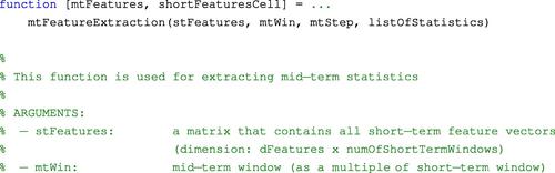
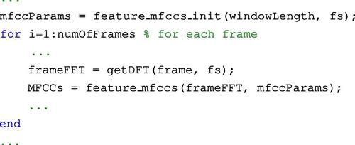
In this line of thinking, function stFeatureExtraction() generates, on a short-term processing basis, 23 features given an audio signal.
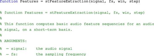
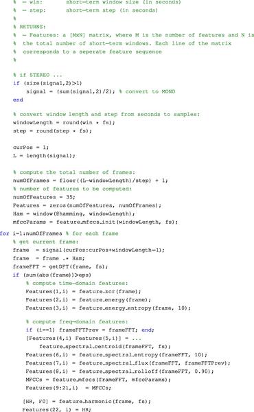
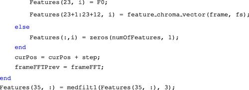
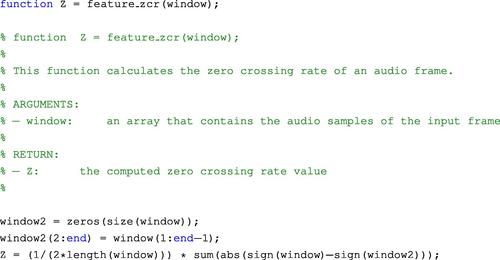
The above function works by breaking the audio input into short-term windows and computing 23 audio features per window. Lines 48–65 call the respective feature extraction functions (which will be described in the next sections). For instance, function feature_zcr() computes the zero-crossing rate of an audio frame.
4.1.2 Mid-Term Windowing in Audio Feature Extraction
Another common technique is the processing of the feature sequence on a mid-term basis. According to this type of processing, the audio signal is first divided into mid-term segments (windows) and then, for each segment, the short-term processing stage is carried out.1 At a next step, the feature sequence, ![]() , which has been extracted from a mid-term segment, is used for computing feature statistics, e.g. the average value of the zero-crossing rate. In the end, each mid-term segment is represented by a set of statistics which correspond to the respective short-term feature sequences. During mid-term processing, we assume that the mid-term segments exhibit homogeneous behavior with respect to audio type and it therefore makes sense to proceed with the extraction of statistics on a segment basis. In practice, the duration of mid-term windows typically lies in the range 1–10 s, depending on the application domain. Figure 4.1 presents the process of extracting mid-term statistics of audio features.
, which has been extracted from a mid-term segment, is used for computing feature statistics, e.g. the average value of the zero-crossing rate. In the end, each mid-term segment is represented by a set of statistics which correspond to the respective short-term feature sequences. During mid-term processing, we assume that the mid-term segments exhibit homogeneous behavior with respect to audio type and it therefore makes sense to proceed with the extraction of statistics on a segment basis. In practice, the duration of mid-term windows typically lies in the range 1–10 s, depending on the application domain. Figure 4.1 presents the process of extracting mid-term statistics of audio features.
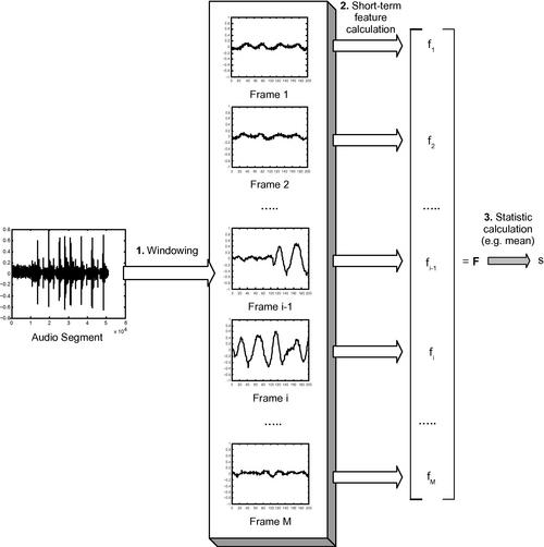
Figure 4.1 Mid-term feature extraction: each mid-term segment is short-term processed and statistics are computed based on the extracted feature sequence.
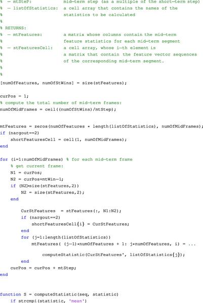
The next function takes as input short-term feature sequences that have been generated by stFeatureExtraction() and returns a vector that contains the resulting feature statistics. If, for example, 23 feature sequences have been computed on a short-term basis and two mid-term statistics are drawn per feature (e.g. the mean value and the standard deviation of the feature), then, the output of the mid-term function is a 46-dimensional vector. The structure of this vector is the following: elements 1 and 24 correspond to the mean and standard deviation of the first short-term feature sequence, elements 2 and 25 correspond to the mean and standard deviation of the second audio short-term sequence, and so on.
4.1.3 Extracting Features from an Audio File
As explained above, function stFeatureExtraction() generates short-term feature sequences from an audio signal, and function mtFeatureExtraction() extracts sequences of mid-term statistics based on the previously extracted short-term features. We will now show how to break a large audio file (or audio stream) into mid-term windows and generate the respective mid-term audio statistics. As shown in Section 2.5, if the audio file to be analyzed has a very long duration, then loading all its content in one step can be prohibitive due to memory issues. This is why function readWavFile() demonstrated how to read progressively the contents of a large audio file using chunks of data (blocks), which can be, for example, one minute long. In the same line of thinking, function featureExtractionFile() is also using data blocks to analyze large audio files. The input arguments of this function are:
• The name of the audio file to be analyzed.
• The short-term window size (in seconds).
• The short-term window step (in seconds).
• The mid-term window size (in seconds).
• The mid-term window step (in seconds).
• A cell array with the names of the feature statistics which will be computed on a mid-term basis.
The arguments at the output of featureExtractionFile() are:
• A matrix, whose rows contain the mid-term sequences of audio statistics. For example, the first row may correspond to the mean value of short-term energy (all features will be explained later in this chapter).
• The time instant that marks the center of each mid-term segment (in seconds).
• A cell array, each element of which contains the short-term feature sequences of the respective mid-term segment.
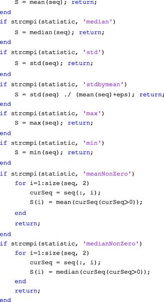
The source code of function featureExtractionFile() is available on the Audio Analysis Library that accompanies the book. We now demonstrate the use of featureExtractionFile() via the example introduced by function plotFeaturesFile():
For example, type:
![]()
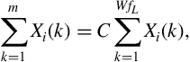
The result will be that the short-term feature sequence of the 6th audio feature and all respective mid-term statistics will be plotted. More specifically, further to the 6th short-term feature sequence, function plotFeaturesFile() will also plot the ![]() statistics, where
statistics, where ![]() is the total number of features and
is the total number of features and ![]() is the number of adopted statistics. In other words, it will plot all the statistics that are relevant to the 6th short-term feature. In this case,
is the number of adopted statistics. In other words, it will plot all the statistics that are relevant to the 6th short-term feature. In this case, ![]() and
and ![]() , therefore, the dimensionality of the final mid-term feature vector is 138. The outcome of the above call to plotFeaturesFile() is presented in Figure 4.2.
, therefore, the dimensionality of the final mid-term feature vector is 138. The outcome of the above call to plotFeaturesFile() is presented in Figure 4.2.
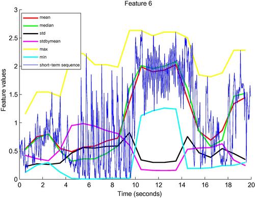
Figure 4.2 Plotting the results of featureExtractionFile(), using plotFeaturesFile(), for the six feature statistics drawn from the 6th adopted audio feature.
4.2 Class Definitions
For the sake of experimentation and as a means to demonstrate the properties of the adopted features and corresponding statistics, we now proceed with two audio analysis examples. The first experimental setup employs audio segments from eight audio classes which are frequently encountered when processing the audio content of movies and radio broadcasts. The second example focuses on music genre classification. Before we proceed with the theoretical and practical descriptions of the audio features, let us briefly present the audio classes that have been involved in our two examples.
The first set of audio classes refers to the problem of detecting/tracking audio events in movies. In the context of content-based processing, the detection of audio events can play an important role in the development of solutions that can deal with important problems, like violence detection in movies and video streams from video sharing sites. In our case, the class names and respective descriptions are summarized in Table 4.1.
Class Descriptions for the Multi-Class Task of Movie Segments
| Class ID | Class Name | Class Description |
| 1 | Music | Music from film soundtracks and music effects |
| 2 | Speech | Speech segments from various speakers, languages, and emotional states. These segments exhibit diverse levels of “noisiness” because speech is usually mixed with other types of audio classes (especially in films soundtracks) |
| 3 | Others1 | Environmental sounds of low energy and practically stable signal intensity (e.g. silence, background noise, wind, rain, etc.) |
| 4 | Others2 | Environmental sounds with abrupt changes in signal energy (e.g. a door closing, the sound of thunder, an object breaking, etc.) |
| 5 | Others3 | High energy, non-abrupt (quasi-repeating) environmental sounds (e.g. machinery) |
| 6 | Gunshots | Gunshots from various gun types. This class contains short, abrupt sounds, and continuous (repetitive) gunshots |
| 7 | Fights | The sounds of humans fighting |
| 8 | Screams | Human screams |
In the second example, we use a set of music tracks to demonstrate the discriminative capability of selected features for the problem of musical genre classification. For pedagogical purposes, we use 360 tracks belonging to three music genres, namely classical, jazz, and electronic (120 samples per class). The reader may also find it interesting to experiment with a popular dataset for music genre classification, i.e. the GTZAN dataset [15], on which several music genre classification algorithms have been tested over the past 10 years.
We now start with the presentation of some of the most important and widely used audio features, along with the corresponding MATLAB code and examples. We also discuss a number of statistics, which, on a mid-term basis, provide acceptable discrimination capability among the audio classes, in the context of the presented examples. Note that we assume that the input to the feature extraction functions is an audio frame and therefore, the functions are to be called inside a short-term analysis process, as it is the case with function stFeatureExtraction(). Similarly, the computation of the mid-term statistics can be encapsulated in functions like mtFeatureExtraction() that operate on consecutive audio segments.
4.3 Time-Domain Audio Features
In general, the time-domain audio features are extracted directly from the samples of the audio signal. Typical examples are the short-term energy and short-term zero-crossing rate. Such features offer a simple way to analyze audio signals, although it is usually necessary to combine them with more sophisticated frequency-domain features, which will be described in Section 4.4. What follows, are definitions of some of the most celebrated time-domain features.
4.3.1 Energy
Let ![]() be the sequence of audio samples of the
be the sequence of audio samples of the ![]() th frame, where
th frame, where ![]() is the length of the frame. The short-term energy is computed according to the equation
is the length of the frame. The short-term energy is computed according to the equation
Usually, energy is normalized by dividing it with ![]() to remove the dependency on the frame length. Therefore, Eq. (4.1) becomes
to remove the dependency on the frame length. Therefore, Eq. (4.1) becomes
Equation (4.2) provides the so-called power of the signal. In the rest of this chapter, we will use the power of the signal in our feature extraction functions but for the sake of simplicity we will keep using the term ‘energy’ in the respective algorithmic descriptions.
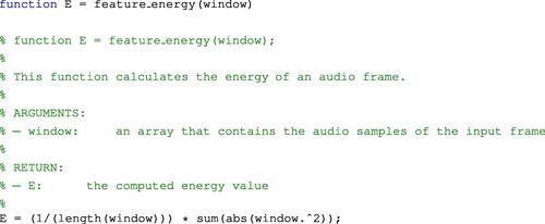
The following function extracts the energy value of a given audio frame:
Short-term energy is expected to exhibit high variation over successive speech frames, i.e. the energy envelope is expected to alternate rapidly between high and low energy states. This can be explained by the fact that speech signals contain weak phonemes and short periods of silence between words. Therefore, a mid-term statistic that can be used for classification purposes in conjunction with short-term energy is the standard deviation ![]() of the energy envelope. An alternative statistic for short-term energy, which is independent of the intensity of the signal, is the standard deviation by mean value ratio,
of the energy envelope. An alternative statistic for short-term energy, which is independent of the intensity of the signal, is the standard deviation by mean value ratio, ![]() [16]. Figure 4.3 presents histograms of the standard deviation by mean ratio for segments of the classes: music and speech. It has been assumed that each segment is homogeneous, i.e. it contains either music or speech. The figure indicates that the values of this statistic are indeed higher for the speech class. The Bayesian error for the respective binary classification task was found to be equal to 17.8% for this experiment, assuming that the two classes are a priori equiprobable and that the likelihood of the statistic (feature) given the class is well approximated using the extracted histograms. Note, that the Bayesian error for the same binary classification task (music vs speech), when the standard deviation statistic is used instead, increases to 37%. Therefore, the normalization of the standard deviation feature by dividing it with the respective mean value provides a crucial performance improvement in this case.
[16]. Figure 4.3 presents histograms of the standard deviation by mean ratio for segments of the classes: music and speech. It has been assumed that each segment is homogeneous, i.e. it contains either music or speech. The figure indicates that the values of this statistic are indeed higher for the speech class. The Bayesian error for the respective binary classification task was found to be equal to 17.8% for this experiment, assuming that the two classes are a priori equiprobable and that the likelihood of the statistic (feature) given the class is well approximated using the extracted histograms. Note, that the Bayesian error for the same binary classification task (music vs speech), when the standard deviation statistic is used instead, increases to 37%. Therefore, the normalization of the standard deviation feature by dividing it with the respective mean value provides a crucial performance improvement in this case.
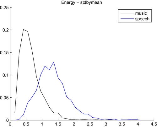
Figure 4.3 Histograms of the standard deviation by mean ratio ![]() of the short-term energy for two classes: music and speech. Speech segments favor higher values of this statistic. The Bayesian error for the respective binary classification task was 17.8%.
of the short-term energy for two classes: music and speech. Speech segments favor higher values of this statistic. The Bayesian error for the respective binary classification task was 17.8%.
4.3.2 Zero-Crossing Rate
The Zero-Crossing Rate (ZCR) of an audio frame is the rate of sign-changes of the signal during the frame. In other words, it is the number of times the signal changes value, from positive to negative and vice versa, divided by the length of the frame. The ZCR is defined according to the following equation:
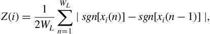
where ![]() is the sign function, i.e.
is the sign function, i.e.

In our toolbox, the computation of the zero-crossing rate for a given frame is implemented in the following m-file:
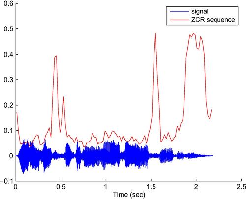
ZCR can be interpreted as a measure of the noisiness of a signal. For example, it usually exhibits higher values in the case of noisy signals. It is also known to reflect, in a rather coarse manner, the spectral characteristics of a signal [17]. Such properties of the ZCR, along with the fact that it is easy to compute, have led to its adoption by numerous applications, including speech-music discrimination [18,16], speech detection [19], and music genre classification [14], to name but a few.
Figure 4.4 presents a speech signal along with the respective ZCR sequence. It shows that the values of ZCR are higher for the noisy parts of the signal, while in speech frames the respective ZCR values are generally lower (depending, of course, on the nature and context of the phoneme that is pronounced each time).
An interesting observation is that the standard deviation of this feature over successive frames is higher for speech signals than for music signal. Indeed, in Figure 4.5 we present the histograms of the standard deviation of ZCR over the short-term frames of music and speech segments. For the generation of these figures, more than 400 segments were used per class. It can be seen that the values of standard deviation are much higher for the speech class. So, in this case, if the standard deviation of the ZCR is used as a mid-term feature for the binary classification task of speech vs music, the respective Bayesian error [5] is equal to 22.3%. If the mean value of the ZCR is used instead, the classification error increases to 34.2%, for this example.
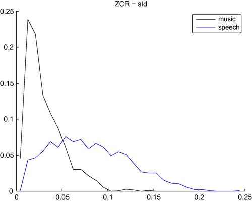
Figure 4.5 Histograms of the standard deviation of the ZCR for music and speech classes. Speech segments yield higher feature values. The respective Bayesian error for this binary classification task is 22.3%.
4.3.3 Entropy of Energy
The short-term entropy of energy can be interpreted as a measure of abrupt changes in the energy level of an audio signal. In order to compute it, we first divide each short-term frame in ![]() sub-frames of fixed duration. Then, for each sub-frame,
sub-frames of fixed duration. Then, for each sub-frame, ![]() , we compute its energy as in Eq. (4.1) and divide it by the total energy,
, we compute its energy as in Eq. (4.1) and divide it by the total energy, ![]() , of the short-term frame. The division operation is a standard procedure and serves as the means to treat the resulting sequence of sub-frame energy values,
, of the short-term frame. The division operation is a standard procedure and serves as the means to treat the resulting sequence of sub-frame energy values, ![]() , as a sequence of probabilities, as in Eq. (4.5):
, as a sequence of probabilities, as in Eq. (4.5):
where
At a final step, the entropy, ![]() of the sequence
of the sequence ![]() is computed according to the equation:
is computed according to the equation:
The following function computes the entropy of energy of a short-term audio frame:
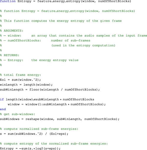
The resulting value is lower if abrupt changes in the energy envelope of the frame exist. This is because, if a sub-frame yields a high energy value, then one of the resulting probabilities will be high, which in turn reduces the entropy of sequence ![]() . Therefore, this feature can be used for the detection of significant energy changes, as it is, for example, the case with the beginning of gunshots, explosions, various environmental sounds, etc. In Figure 4.6, an example of the sequence of entropy values is presented for an audio signal that contains three gunshots. It can be seen that in the beginning of each gunshot the value of this feature decreases. Several research efforts have experimented with the entropy of energy in the context of detecting the onset of abrupt sounds, e.g. [20, 21].
. Therefore, this feature can be used for the detection of significant energy changes, as it is, for example, the case with the beginning of gunshots, explosions, various environmental sounds, etc. In Figure 4.6, an example of the sequence of entropy values is presented for an audio signal that contains three gunshots. It can be seen that in the beginning of each gunshot the value of this feature decreases. Several research efforts have experimented with the entropy of energy in the context of detecting the onset of abrupt sounds, e.g. [20, 21].
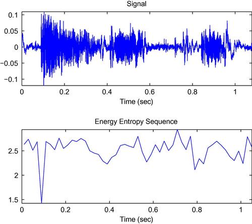
Figure 4.6 Sequence of entropy values for an audio signal that contains the sounds of three gunshots. Low values appear at the onset of each gunshot.
Figure 4.7 presents a second example, which is based on computing a long-term statistic of this feature for segments belonging to the three musical genres that were previously examined. Specifically, for each music segment, we have selected the minimum of the sequence of entropy values as the long-term feature that will eventually be used to discriminate among genres. It can be seen that this long-term feature takes lower values for electronic music and higher values for classical music (although a similar conclusion cannot be reached for Jazz). This can be partly explained by the fact that electronic music tends to contain many abrupt energy changes (low entropy), compared to classical music, which exhibits a smoother energy profile. The reader is reminded that such examples serve pedagogical needs and do not imply that the adopted features are optimal in any sense or that they can necessarily lead to acceptable performance in a real-world scenario.
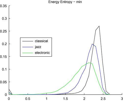
Figure 4.7 Histograms of the minimum value of the entropy of energy for audio segments from the genres of jazz, classical and electronic music. The Bayesian error for this three-class classification task, using just this single feature, was equal to 44.8%.
4.4 Frequency-Domain Audio Features
As discussed in Section 3.1, the Discrete Fourier Transform (DFT) of a signal can be easily computed with MATLAB using the built-in function fft(). DFT is widely used in audio signal analysis because it provides a convenient representation of the distribution of the frequency content of sounds, i.e. of the sound spectrum. We will now describe some widely used audio features that are based on the DFT of the audio signal. Features of this type are also called frequency-domain (or spectral) audio features.
In order to compute the spectral features, we must first compute the DFT of the audio frames using the getDFT() function (Section 3.1). Function stFeatureExtraction(), which has already been described in 4.1, computes the DFT of each audio frame (calling function getDFT()), and the resulting DFT coefficients are used to compute various spectral features. In order to proceed, let ![]() , be the magnitude of the DFT coefficients of the
, be the magnitude of the DFT coefficients of the ![]() th audio frame (at the output of function getDFT()). In the following paragraphs, we will describe how the respective spectral features are computed based on the DFT coefficients of the audio frame.
th audio frame (at the output of function getDFT()). In the following paragraphs, we will describe how the respective spectral features are computed based on the DFT coefficients of the audio frame.
Note: ![]() is the number of samples per short-term window (frame). This is also the number of DFT coefficients of the frame. Roughly speaking, for the computation of spectral features, it suffices to work with the first half of the coefficients, because the second half mainly serves to reconstruct the original signal. For notational simplicity, let
is the number of samples per short-term window (frame). This is also the number of DFT coefficients of the frame. Roughly speaking, for the computation of spectral features, it suffices to work with the first half of the coefficients, because the second half mainly serves to reconstruct the original signal. For notational simplicity, let ![]() be the number of coefficients that are used in the computations to follow.
be the number of coefficients that are used in the computations to follow.
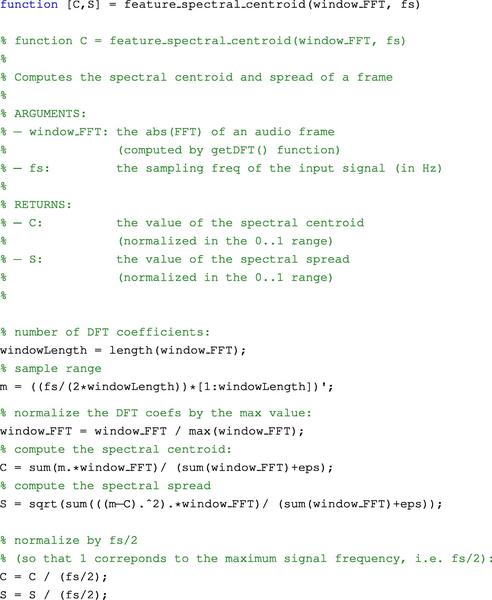
4.4.1 Spectral Centroid and Spread
The spectral centroid and the spectral spread are two simple measures of spectral position and shape. The spectral centroid is the center of ‘gravity’ of the spectrum. The value of spectral centroid, ![]() , of the
, of the ![]() th audio frame is defined as:
th audio frame is defined as:
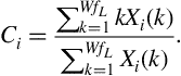
Spectral spread is the second central moment of the spectrum. In order to compute it, one has to take the deviation of the spectrum from the spectral centroid, according to the following equation:
The MATLAB code that computes the spectral centroid and spectral spread of an audio frame is presented in the following function. Note that this function (like all spectral-based functions of this chapter) takes as input the magnitude of the DFT coefficients of an audio frame (output of the getDFT() function), instead of the audio frame itself. The reader is prompted to revisit Section 4.1 and in particular the stFeatureExtraction() function, in order to study how the DFT and related spectral features are computed on a short-term basis. Finally, we normalize both features in the range [0, 1], by dividing their values by ![]() . This type of normalization can be very useful when features that take frequency values are combined with other features in audio analysis tasks.
. This type of normalization can be very useful when features that take frequency values are combined with other features in audio analysis tasks.
Returning to the spectral centroid, it can be observed that higher values correspond to brighter sounds. In Figure 4.8, we present the histograms of the maximum value of the spectral centroid for audio segments from three classes of environmental sounds. It can be seen that the class ‘others1,’ which mostly consists of background noise, silence, etc. exhibits lower values for this statistic, while the respective values are higher for the abrupt sounds of classes “others2” and “others3”.
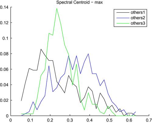
Figure 4.8 Histograms of the maximum value of the sequence of values of the spectral centroid, for audio segments from three classes of environmental sounds: others1, others2, and others3. The Bayesian error for this three-class task, using this single feature, was equal to 44.6%.
On the other hand, spectral spread measures how the spectrum is distributed around its centroid. Obviously, low values of the spectral spread correspond to signals whose spectrum is tightly concentrated around the spectral centroid. In Figure 4.9, we present the histograms of the maximum value (mid-term statistic) of the sequence of values of the spectral spread feature for audio segments that stem from three musical classes (classical, jazz, and electronic). In this specific example, the results indicate that the spectrograms of excerpts of electronic music are (usually) more widely spread around their centroid than (especially) classical and jazz music. It should not be taken for granted that this observation is the same for every music track in these genres.
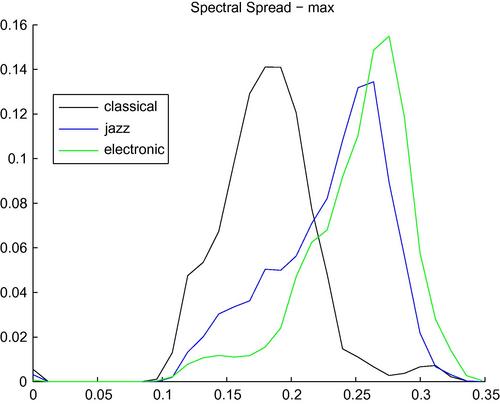
Figure 4.9 Histograms of the maximum value of the sequences of the spectral spread feature, for audio segments from three music genres: classical, jazz, and electronic. The Bayesian error for this three-class classification task, using this single feature, was found to be equal to 41.8%.
4.4.2 Spectral Entropy
Spectral entropy [22] is computed in a similar manner to the entropy of energy, although, this time, the computation takes place in the frequency domain. More specifically, we first divide the spectrum of the short-term frame into ![]() sub-bands (bins). The energy
sub-bands (bins). The energy ![]() of the
of the ![]() th sub-band,
th sub-band, ![]() , is then normalized by the total spectral energy, that is,
, is then normalized by the total spectral energy, that is, ![]() . The entropy of the normalized spectral energy
. The entropy of the normalized spectral energy ![]() is finally computed according to the equation:
is finally computed according to the equation:
The function that implements the spectral entropy is as follows:
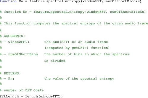
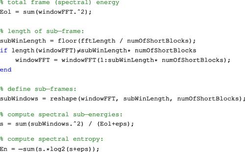
Figure 4.10 presents the histograms of the standard deviation of sequences of spectral entropy of segments from three classes: music, speech, and others1 (low-level environmental sounds). It can be seen that this statistic has lower values for the environmental sounds, while speech segments yield the highest values among the three classes.
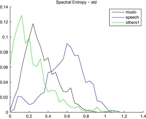
Figure 4.10 Histograms of the standard deviation of sequences of the spectral entropy feature, for audio segments from three classes: music, speech, and others1 (low-level environmental sounds).
A variant of spectral entropy called chromatic entropy has been used in [23] and [24] in order to efficiently discriminate between speech and music.
4.4.3 Spectral Flux
Spectral flux measures the spectral change between two successive frames and is computed as the squared difference between the normalized magnitudes of the spectra of the two successive short-term windows:
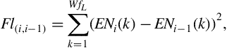
where ![]() , i.e.
, i.e. ![]() is the
is the ![]() th normalized DFT coefficient at the
th normalized DFT coefficient at the ![]() th frame. The spectral flux has been implemented in the following function:
th frame. The spectral flux has been implemented in the following function:
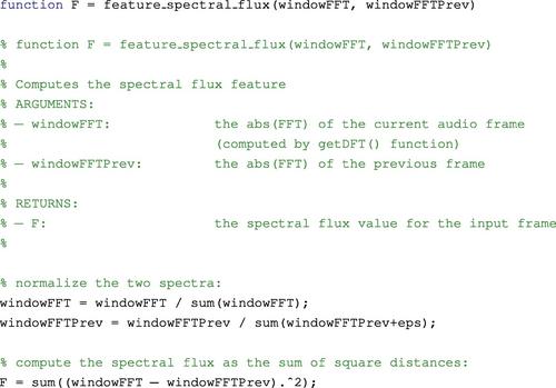
Figure 4.11 presents the histograms of the mean value of the spectral flux sequences of segments from two classes: music and speech. It can be seen that the values of spectral flux are higher for the speech class. This is expected considering that local spectral changes are more frequent in speech signals due to the rapid alternation among phonemes, some of which are quasi-periodic, whereas others are of a noisy nature.
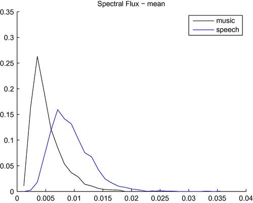
Figure 4.11 Histograms of the mean value of sequences of spectral flux values, for audio segments from two classes: music and speech.
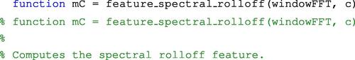
4.4.4 Spectral Rolloff
This feature is defined as the frequency below which a certain percentage (usually around 90%) of the magnitude distribution of the spectrum is concentrated. Therefore, if the ![]() th DFT coefficient corresponds to the spectral rolloff of the
th DFT coefficient corresponds to the spectral rolloff of the ![]() th frame, then it satisfies the following equation:
th frame, then it satisfies the following equation:
where ![]() is the adopted percentage (user parameter). The spectral rolloff frequency is usually normalized by dividing it with
is the adopted percentage (user parameter). The spectral rolloff frequency is usually normalized by dividing it with ![]() , so that it takes values between 0 and 1. This type of normalization implies that a value of 1 corresponds to the maximum frequency of the signal, i.e. to half the sampling frequency. The MATLAB function that implements this feature, given the DFT spectrum of a frame, is the following:
, so that it takes values between 0 and 1. This type of normalization implies that a value of 1 corresponds to the maximum frequency of the signal, i.e. to half the sampling frequency. The MATLAB function that implements this feature, given the DFT spectrum of a frame, is the following:
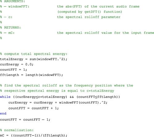
Spectral rolloff can be also treated as a spectral shape descriptor of an audio signal and can be used for discriminating between voiced and unvoiced sounds [7,5]. It can also be used to discriminate between different types of music tracks. Figure 4.12 presents an example of a spectral rolloff sequence. In order to generate this figure, we created a synthetic music track (20 s long) consisting of four different music excerpts (5 s each). The first part of the synthetic track stems from classical music, the second and third parts originate from two different electronic tracks, while the final part comes from a jazz track. It can be easily observed that the electronic music tracks correspond to higher values of the spectral rolloff sequence. In addition, the variation is more intense for this type of music. This is to be expected, if we consider the shape of the respective spectrograms: in the classical and jazz parts, most of the spectral energy is concentrated in lower frequencies and only some harmonics can be seen in the middle and higher frequency regions. On the other hand, in this example, electronic music yields a wider spectrum and as a consequence, the respective spectral rolloff values are higher.
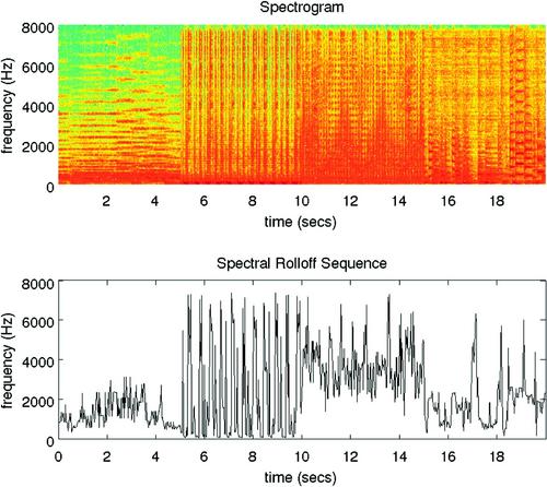
Figure 4.12 Example of the spectral rolloff sequence of an audio signal that consists of four music excerpts. The first 5 s stem from a classical music track. Seconds 5–10 and 10–15 contain two different segments of electronic music, while the last 5 s contain a jazz part. It is readily observed that the segments of electronic music yield higher values of the spectral rolloff feature because the respective spectra exhibit a wider distribution.
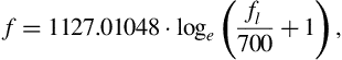
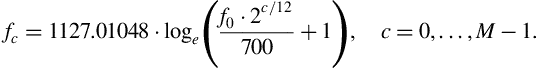
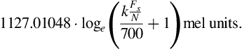
4.4.5 MFCCs
Mel-Frequency Cepstrum Coefficients (MFCCs) have been very popular in the field of speech processing [5]. MFCCs are actually a type of cepstral representation of the signal, where the frequency bands are distributed according to the mel-scale, instead of the linearly spaced approach. In order to extract MFCCs from a frame, the following steps are executed:
1. The DFT is computed.
2. The resulting spectrum is given as input to a mel-scale filter bank that consists of ![]() filters. The filters usually have overlapping triangular frequency responses. The mel-scale introduces a frequency warping effect in an attempt to conform with certain psychoacoustic observations [25] which have indicated that the human auditory system can distinguish neighboring frequencies more easily in the low-frequency region. Over the years a number of frequency warping functions have been proposed, e.g.,
filters. The filters usually have overlapping triangular frequency responses. The mel-scale introduces a frequency warping effect in an attempt to conform with certain psychoacoustic observations [25] which have indicated that the human auditory system can distinguish neighboring frequencies more easily in the low-frequency region. Over the years a number of frequency warping functions have been proposed, e.g.,
![]()
[26]. This equation is presented in Figure 4.13. In other words, the mel scale is a perceptually motivated scale of frequency intervals, which, if judged by a human listener, are perceived to be equally spaced.
3. If ![]() , is the power at the output of the
, is the power at the output of the ![]() th filter, then the resulting MFCCs are given by the equation
th filter, then the resulting MFCCs are given by the equation
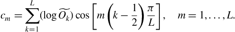
Therefore, according to Eq. (4.13), MFCCs are the discrete cosine transform coefficients of the mel-scaled log-power spectrum.
MFCCs have been widely used in speech recognition [27], musical genre classification [14], speaker clustering [28], and many other audio analysis applications.
In this book we have adopted the implementation proposed by Slaney in [29]. In order to improve computational complexity, we have added a function that precomputes the basic quantities involved in the computation of the MFCCs, i.e. the weights of the triangular filters and the DCT matrix. The function that implements this preprocessing step is the following:
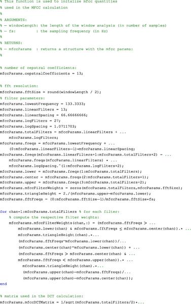
![]()
The above function returns a structure that contains the MFCC parameters which are then used to compute the MFCCs. The final MFCC values for each short-term frame (assuming that the DFT has already been extracted) are achieved by calling the following function:
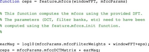
The reader can refer to the code of the stFeatureExtraction() function (Section 4.1) to understand how the mfcc function must be called in the context of the short-term analysis process. We review this process in the following lines:
The MFCCs have proved to be powerful features in several audio analysis applications. For instance, in the binary classification task of speech vs music, they exhibit significant discriminative capability. Figure 4.14 presents the histograms of the standard deviation of the 2nd MFCC for the binary classification task of speech vs music. It can be seen that the discriminative power of this feature is quite high, and that the estimated Bayesian error is equal to 11.8% using this single feature statistic. It is worth noting that, depending on the task at hand, different subsets of the MFCCs have been used over the years. For example, it has become customary in many music processing applications to select the first 13 MFCCs because they are considered to carry enough discriminative information in the context of various classification tasks.
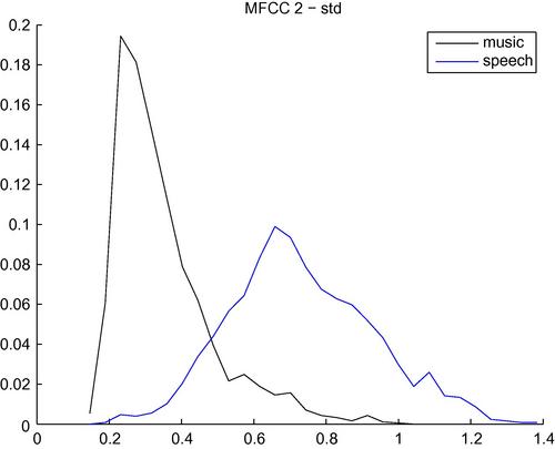
Figure 4.14 Histograms of the standard deviation of the 2nd MFCC for the classes of music and speech. The estimated Bayesian error is equal to 11.8% using this single feature statistic.
4.4.6 Chroma Vector
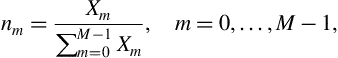
The chroma vector is a 12-element representation of the spectral energy of proposed in [30]. This is a widely used descriptor, mostly in music-related applications [31,32,33,24].
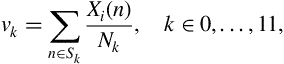
The chroma vector is computed by grouping the DFT coefficients of a short-term window into 12 bins. Each bin represents one of the 12 equal-tempered pitch classes of Western-type music (semitone spacing). Each bin produces the mean of log-magnitudes of the respective DFT coefficients:
where ![]() is a subset of the frequencies that correspond to the DFT coefficients and
is a subset of the frequencies that correspond to the DFT coefficients and ![]() is the cardinality of
is the cardinality of ![]() . In the context of a short-term feature extraction procedure, the chroma vector,
. In the context of a short-term feature extraction procedure, the chroma vector, ![]() , is usually computed on a short-term frame basis. This results in a matrix,
, is usually computed on a short-term frame basis. This results in a matrix, ![]() , with elements
, with elements ![]() , where indices
, where indices ![]() and
and ![]() represent pitch class and frame number, respectively.
represent pitch class and frame number, respectively. ![]() is actually a matrix representation of the sequence of chroma vectors and is also known as the chromagram (in an analogy to the spectrogram).
is actually a matrix representation of the sequence of chroma vectors and is also known as the chromagram (in an analogy to the spectrogram).
In Figure 4.15 we provide two examples of chromagrams, for a music and a speech segment. There is an obvious difference between the two cases: the music chromogram is strongly characterized by two (or three) dominant coefficients, with all other chroma elements having values close to zero. It can also be observed that these dominant chroma coefficients are quite ‘stable’ for a short period of time in music signals. On the other hand, the chroma coefficients are noisier for speech segments (e.g. Figure 4.15b). This difference in the behavior of the chroma vector among speech and music signals has been used in speech-music discrimination applications, e.g. [24].
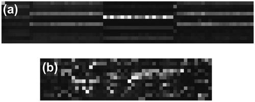
Figure 4.15 Chromagrams for a music and a speech segment. The chromagram of music is characterized by a small number of dominant coefficients, which are stable for a short-time duration. On the other hand, chromagrams of speech are generally noisier.
In our toolbox, the chroma vector of an audio frame is extracted using function feature_chroma_vector().
4.5 Periodicity Estimation and Harmonic Ratio
Audio signals can be broadly categorized as quasi-periodic and aperiodic (noise-like). The term ‘quasi-periodic’ refers to the fact that although some signals exhibit periodic behavior, it is extremely hard to find two signal periods that are exactly the same (by inspecting the signal on a sample basis). Quasi-periodic signals include voiced phonemes and the majority of music signals. On the other hand, noise-like signals include unvoiced phonemes, background/environmental noise, applause, gunshots, etc. It has to be noted that there are, of course, gray areas in this categorization, as is, for example, the case with fricative phonemes and some percussive sounds. For the sake of simplicity, we will refer to the quasi-periodic sounds as periodic. For this type of signal, the frequency equivalent of the length of the (fundamental) period of the signal is the so-called fundamental frequency and the algorithms that attempt to estimate this frequency are called fundamental frequency tracking algorithms. Note that, in the literature, the term ‘pitch’ is often used interchangeably with the term fundamental frequency. Strictly speaking, pitch represents perceived frequency, like loudness represents perceived signal intensity. However, in many cases, fundamental frequency and pitch coincide, hence the simplification.
A popular, simple technique for estimating the fundamental period is based on the autocorrelation function [8]. According to this method, the signal is shifted and for each signal shift (lag) the correlation (resemblance) of the shifted signal with the original one is computed. In the end, we choose the fundamental period to be the lag, for which the signal best resembles itself, i.e. where the autocorrelation is maximized. We now provide a more detailed description of the algorithmic steps that lead to the estimation of the fundamental frequency based on the autocorrelation function. Our approach follows the guidelines set in the MPEG-7 audio description scheme [34]:
1. Compute the autocorrelation function for frame ![]() , as in the following equation:
, as in the following equation:
where ![]() is the number of samples per frame. In other words
is the number of samples per frame. In other words ![]() corresponds to the correlation of the
corresponds to the correlation of the ![]() th frame with itself at time-lag
th frame with itself at time-lag ![]() .
.
2. Normalize the autocorrelation function:
3. Compute the maximum value of ![]() (also known as the harmonic ratio):
(also known as the harmonic ratio):
![]() and
and ![]() stand for the minimum and maximum allowable values of the fundamental period.
stand for the minimum and maximum allowable values of the fundamental period. ![]() is often defined by the user, whereas
is often defined by the user, whereas ![]() usually corresponds to the lag for which the first zero crossing of
usually corresponds to the lag for which the first zero crossing of ![]() occurs. The harmonic ratio can be also used as a feature to discriminate between voiced and unvoiced sounds.
occurs. The harmonic ratio can be also used as a feature to discriminate between voiced and unvoiced sounds.
4. Finally, the fundamental period is selected as the position where the maximum value of ![]() occurs:
occurs:
The fundamental frequency is then:

As an example, consider the following periodic signal:
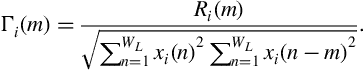
The number of samples is ![]() and the sampling frequency is 16 kHz. Figure 4.16 presents the autocorrelation and normalized autocorrelation functions of this signal. The position of the maximum normalized autocorrelation value defines the fundamental period.
and the sampling frequency is 16 kHz. Figure 4.16 presents the autocorrelation and normalized autocorrelation functions of this signal. The position of the maximum normalized autocorrelation value defines the fundamental period.
Figure 4.16 Autocorrelation, normalized autocorrelation, and detected peak for a periodic signal. The position (32) of the maximum value of the normalized autocorrelation function corresponds to the fundamental period ![]() . Therefore, the fundamental frequency is
. Therefore, the fundamental frequency is ![]() . The maximum value itself is the harmonic ratio.
. The maximum value itself is the harmonic ratio.
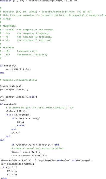
The code that implements the fundamental frequency estimation (along with the harmonic ratio) is the following:
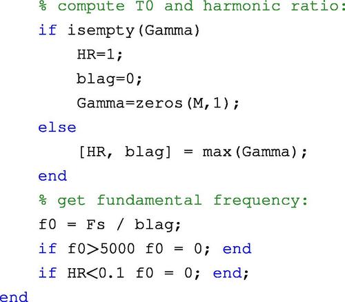
In Figure 4.17, we demonstrate the discriminative power of the harmonic ratio. In particular, we present the histograms of the maximum value of the harmonic ratio for two classes: speech and others1 (noisy environmental sounds). It can be seen that the adopted statistic takes much higher values for the speech class compared to the noisy class, as is expected. In particular, a binary classifier can achieve up to 88% performance using this single feature.
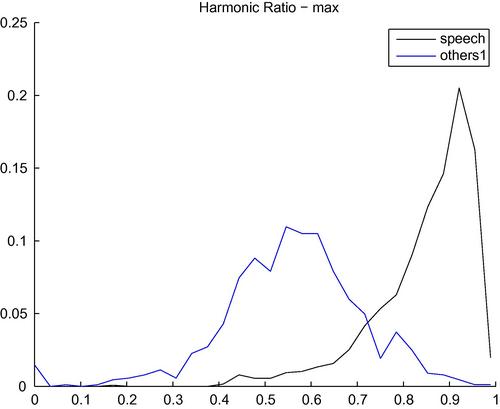
Figure 4.17 Histograms of the maximum value of sequences of values of the harmonic ratio for two classes of sounds (speech and others1). The estimated Bayesian error for this binary classification task is 12.1%.
Remarks
• In feature_harmonic() we have used the zero-crossing rate feature in order to estimate the number of peaks in the autocorrelation sequence. Too many peaks indicate that the signal is not periodic. Two other constraints during the computation of the fundamental frequency are associated with the minimum allowable value for the harmonic ratio and the range of allowable values for the fundamental frequency. These values are usually empirically set depending on the application. For example, if we are interested in computing the pitch value of speech signals (e.g. of male speakers), then the range of values of the fundamental frequency should be quite narrow (e.g. 80–200 Hz).
• Fundamental frequency estimation is a difficult task. Therefore, it is no surprise that several spectral methods have also been proposed in the literature, in addition to the popular autocorrelation approach. Some of the exercises at the end of this chapter introduce the key algorithmic concepts of selected frequency-based methods and challenge the reader to proceed with their implementation.
4.6 Exercises
1. (D03) Write a MATLAB function that:
(a) Uses audiorecorder to record a number of audio segments, 0.5s each. Section 2.6.2 demonstrates how this can be achieved.
(b) For each recorded segment, computes and plots (on two separate subfigures) the sequences of the short-time energy and zero-crossing rate features. Adopt a 20 ms frame.
Note that this process must fit in an online mode of operation.
2. (D04) One of the earliest methods in speech processing for the estimation of the fundamental frequency of speech signals has been the work of Schroeder [35]. Schroeder’s method was based on the idea that although the fundamental frequency may not correspond to the highest peak in the spectrum of the signal, it can emerge as the common divisor of its harmonic frequencies. As a matter of fact, the method can even trace the fundamental frequency when it is not present in the signal at all. This line of thinking led to the generation from the speech signal of the so-called “frequency histogram” and its generalization, the “harmonic product spectrum.” In this exercise, we provide a simplified version of Schroeder’s algorithm based on the DFT of the signal. Assume that the signal is short-term processed and focus on a single frame. Follow the steps below:
• Step 1: Compute the log-magnitude of the DFT coefficients of the frame.
• Step 2: Detect all spectral peaks and mark the corresponding frequencies. Let ![]() be the resulting set, where
be the resulting set, where ![]() is a frequency,
is a frequency, ![]() the magnitude of the respective spectral peak, and
the magnitude of the respective spectral peak, and ![]() the number of detected peaks. To simplify the pairs in
the number of detected peaks. To simplify the pairs in ![]() are sorted in ascending order with respect to frequency. Hint: You may find it useful to employ MATLAB’s function findpeaks() (http://www.mathworks.com/help/signal/ref/findpeaks.html
are sorted in ascending order with respect to frequency. Hint: You may find it useful to employ MATLAB’s function findpeaks() (http://www.mathworks.com/help/signal/ref/findpeaks.html![]() ) to detect the spectral peaks.
) to detect the spectral peaks.
• Step 3: Select ![]() and
and ![]() such that
such that ![]() is the allowable range of fundamental frequencies for the task at hand.
is the allowable range of fundamental frequencies for the task at hand.
• Step 4: Initialize a histogram by placing each ![]() at the center of a bin, if
at the center of a bin, if ![]() . The height of each bin is set equal to the log-magnitude of the DFT coefficient that corresponds to
. The height of each bin is set equal to the log-magnitude of the DFT coefficient that corresponds to ![]() .
.
• Step 5: For each ![]() in
in ![]() compute its submultiples in the range
compute its submultiples in the range ![]() . Place each submultiple in the correct bin and increase the height of the bin by the log-magnitude of
. Place each submultiple in the correct bin and increase the height of the bin by the log-magnitude of ![]() , i.e. of the frequency from which the submultiple originated. The correct bin is chosen based on the proximity of the submultiple to the bin centers.
, i.e. of the frequency from which the submultiple originated. The correct bin is chosen based on the proximity of the submultiple to the bin centers.
• Step 6: Select the bin with the highest accumulated magnitude. The frequency at the center of the bin is the detected fundamental frequency.
Provide a MATLAB implementation of the above algorithmic description and compare the results with the autocorrelation method that was presented earlier in this chapter. Run your program on a signal from a single speaker, then for a monophonic music signal, and finally on an excerpt from a polyphonic track. In which case is the resulting pitch-tracking sequence the noisiest? Comment on your findings.
3. (D04) In this exercise you are asked to implement a variant of an MPEG-7 audio descriptor, the Audio Spectrum Envelope (ASE), which forms the basis for computing several other spectral descriptors in MPEG-7. The basic idea behind the ASE feature is that the frequency of 1000 Hz is considered to be the center of hearing and that the spectrum is divided into logarithmically distributed frequency bands around 1000 Hz. To compute the proposed variant of the ASE on a short-term frame basis, implement the following steps:
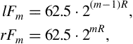
• Step 1: At the first step, the resolution, ![]() , of the frequency bands is defined (as a fraction of the octave) using the equation
, of the frequency bands is defined (as a fraction of the octave) using the equation
![]()
This equation implies that ![]() can take the following eight discrete values:
can take the following eight discrete values: ![]() . For example, the value
. For example, the value ![]() means that the width of each frequency band is equal to
means that the width of each frequency band is equal to ![]() th of the octave.
th of the octave.
• Step 2: The next step is to define the edges of the frequency bands. To this end, it is first assumed that the frequencies 62.5 Hz and 16 kHz are the lower and upper limits of human hearing, respectively. Then, starting from the lower limit of hearing, the left and right edges of each frequency band are computed as follows:
where ![]() are the left and right edges of the
are the left and right edges of the ![]() th frequency band,
th frequency band, ![]() ; and
; and ![]() is the number of frequency bands covering the frequency range
is the number of frequency bands covering the frequency range ![]() . For example, if
. For example, if ![]() , then
, then ![]() and the first frequency band covers the frequency range
and the first frequency band covers the frequency range ![]() . Similarly, the last frequency band
. Similarly, the last frequency band ![]() covers the frequency range
covers the frequency range ![]() . Note, that the smaller the value of
. Note, that the smaller the value of ![]() , the more narrow the frequency band. However, if you place the band edges on a logarithmic scale, you will readily observe that each band is always
, the more narrow the frequency band. However, if you place the band edges on a logarithmic scale, you will readily observe that each band is always ![]() octaves wide. Furthermore, for this specific example, if
octaves wide. Furthermore, for this specific example, if ![]() and
and ![]() , the respective frequency bands are
, the respective frequency bands are ![]() and
and ![]() , i.e. the center of hearing is the right edge of the 16th band and the left edge of the 17th band.
, i.e. the center of hearing is the right edge of the 16th band and the left edge of the 17th band.
• Step 3: Compute the magnitude of the DFT coefficients of the frame. It is, of course, assumed that you have already decided on the frame length. Note that, until the previous step, all computations conformed with the MPEG-7 standard. However, this step has introduced a variation to the implementation of this MPEG-7 descriptor because we are using the magnitude of the DFT coefficients instead of the ‘power spectrum’ that MPEG-7 offers [34].
• Step 4: Assign each DFT coefficient to the respective frequency band. If a coefficient should fall exactly on the boundary between successive bands, then it is assigned to the leftmost band. Associate a total magnitude with each band. Whenever a DFT coefficient is assigned to a band, increase the cumulative magnitude by the magnitude of the DFT coefficient.
• Step 5: Finally, repeat the previous step for all coefficients in the range ![]() and
and ![]() , where
, where ![]() is the sampling rate.
is the sampling rate.
The outcome of the above procedure is a vector of ![]() coefficients. This vector can also be treated as a bin representation of the spectrum or as an envelope (hence, the name, ASE), in the sense that it provides a simplified spectrum representation. Obviously, the smaller the value of
coefficients. This vector can also be treated as a bin representation of the spectrum or as an envelope (hence, the name, ASE), in the sense that it provides a simplified spectrum representation. Obviously, the smaller the value of ![]() the more detailed the resulting envelop, i.e. parameter
the more detailed the resulting envelop, i.e. parameter ![]() provides the means to control the resolution of the representation. After you implement the proposed variant as an m-file, apply it on various sounds of your choice. Experiment with
provides the means to control the resolution of the representation. After you implement the proposed variant as an m-file, apply it on various sounds of your choice. Experiment with ![]() in order to get a better understanding of the concept of varying spectral resolution. Can you modify function stFeatureExtraction() to add the functionality of this feature?
in order to get a better understanding of the concept of varying spectral resolution. Can you modify function stFeatureExtraction() to add the functionality of this feature?
4. (D03) Another old-but-popular fundamental frequency tracking technique is the Average Magnitude Difference Function (AMDF) [36]. This method was born in the mid-1970s, out of the need to reduce the computational burden of the autocorrelation approach, which is heavily based on multiplications (see Eq. (4.15)). The key idea behind the AMDF method is that if ![]() , is an audio frame and
, is an audio frame and ![]() is the length of its period in samples, then the sum of absolute differences between the samples of
is the length of its period in samples, then the sum of absolute differences between the samples of ![]() and the samples of its shifted version by
and the samples of its shifted version by ![]() should be approximately equal to zero (remember that we are dealing with pseudo-periodic signals, hence, the word ‘approximately’). We can therefore define the AMDF at time-lag
should be approximately equal to zero (remember that we are dealing with pseudo-periodic signals, hence, the word ‘approximately’). We can therefore define the AMDF at time-lag ![]() as
as
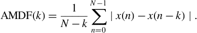
The above equation is computed for all the values of ![]() whose equivalent frequency lies in the desired frequency range. We then seek the global minimum (usually beyond the first zero crossing of the AMDF). The lag which corresponds to this global minimum is the length of the period in samples.
whose equivalent frequency lies in the desired frequency range. We then seek the global minimum (usually beyond the first zero crossing of the AMDF). The lag which corresponds to this global minimum is the length of the period in samples.
In this exercise you are asked to implement the AMDF function, apply it on signals of your choice, and compare the resulting pitch sequences with those of the autocorrelation-based approach in Section 4.5.
5. (D04) This exercise revolves around a variant of spectral entropy (Section 4.4.2), the chromatic entropy, which was introduced in [24]. To compute this feature on a short-term frame basis, do the following:
• Step 1: Let ![]() be the frequency range of interest, where
be the frequency range of interest, where ![]() is the maximum frequency and
is the maximum frequency and ![]() , where
, where ![]() is the sampling frequency.
is the sampling frequency.
• Step 2: All computations are then carried out on a mel-scale. Specifically, the frequency axis is warped according to the equation
where ![]() is the frequency on a linear axis.
is the frequency on a linear axis.
• Step 3: Split the mel-scaled frequency range into bands. The centers, ![]() , of the bands coincide with the semitones of the equal-tempered chromatic scale. If, for the moment, frequency warping is ignored, the centers follow the equation:
, of the bands coincide with the semitones of the equal-tempered chromatic scale. If, for the moment, frequency warping is ignored, the centers follow the equation:
where ![]() is a starting frequency (13.75 Hz in this case) and
is a starting frequency (13.75 Hz in this case) and ![]() is the number of bands. Given that we use a frequency warped axis, we need to combine Eqs. (4.22) and (4.23) to form
is the number of bands. Given that we use a frequency warped axis, we need to combine Eqs. (4.22) and (4.23) to form
• Step 4: Compute the DFT of the frame. Assign each DFT coefficient to a band after detecting the closest band center. Remember that the ![]() th DFT coefficient corresponds to frequency
th DFT coefficient corresponds to frequency ![]() , where
, where ![]() is the length of the frame. Therefore, on a mel-scale, the
is the length of the frame. Therefore, on a mel-scale, the ![]() th coefficient is located at
th coefficient is located at
If a DFT coefficient is assigned to the ![]() th frequency band, its magnitude is added to the respective sum of magnitudes,
th frequency band, its magnitude is added to the respective sum of magnitudes, ![]() , of the band.
, of the band.
• Step 5: Each ![]() is then normalized as follows:
is then normalized as follows:
where ![]() is the normalized version of
is the normalized version of ![]() .
.
• Step 6: Due to the way Eq. (4.25) is defined, the ![]() s can also be interpreted as probabilities. Therefore, in this final step, the entropy,
s can also be interpreted as probabilities. Therefore, in this final step, the entropy, ![]() , of sequence
, of sequence ![]() , is computed:
, is computed:
Implement the above feature extraction procedure as an m-file and apply it to an excerpt of classical music and to the speech signal of a single speaker. What can you observe in terms of the standard deviation of this feature over the short-term frames of the two segments?
6. (D05) As the reader may have already suspected, a significant body of pitch-tracking literature revolves around the autocorrelation method. An interesting idea that can also be applied in the context of multipitch analysis of audio signals is introduced in [37], where a generalized autocorrelation method is proposed.
In this exercise, you are asked to provide an approximate implementation of the key processing stages of the work in [37]. More specifically, you will first implement the Summary Autocorrelation Function (SACF) of an audio frame and then the Enhanced Summary Autocorrelation Function (ESAFC) of the frame. To this end, let ![]() be an audio frame. Use the following steps:
be an audio frame. Use the following steps:
• Step 1: Create a lowpass filter ![]() , with a cutoff frequency at 1 kHZ.
, with a cutoff frequency at 1 kHZ.
• Step 2: Create a highpass filter, ![]() , with a cutoff frequency at 1 kHZ. Both filters should exhibit a 12 dB/octave attenuation at the stopband.
, with a cutoff frequency at 1 kHZ. Both filters should exhibit a 12 dB/octave attenuation at the stopband.
• Step 3: Filter ![]() with
with ![]() . Let
. Let ![]() be the resulting signal.
be the resulting signal.
• Step 4: Filter ![]() with
with ![]() . The output of
. The output of ![]() is first half-wave rectified and then lowpass filtered with
is first half-wave rectified and then lowpass filtered with ![]() . Let
. Let ![]() be the resulting signal.
be the resulting signal.
• Step 5: Let ![]() and
and ![]() be the magnitude of the DFT of
be the magnitude of the DFT of ![]() and
and ![]() , respectively. Implement the equation:
, respectively. Implement the equation:
where ![]() is a user parameter and
is a user parameter and ![]() . The resulting signal,
. The resulting signal, ![]() , is the SACF. with
, is the SACF. with ![]() and compare the SACF with the standard autocorrelation. What do you observe when
and compare the SACF with the standard autocorrelation. What do you observe when ![]() , and what is the effect of
, and what is the effect of ![]() ?
?
• Step 6: Clip the SACF to positive values, time-scale it by a factor of 2, subtract the result from the original SACF, and clip the result of the subtraction to positive values. What is the effect of this operation?
• Step 7: You can repeat the previous step for a time-scaling factor of three, four, etc.
The outcome of Step 6 (possibly combined with [optional] Step 7) is the Enhanced Summary Autocorrelation Function (ESACF). After you implement the ESACF, apply it on a short-term processing basis on a music signal of two instruments and a speech signal of two voices. What are your conclusions if you place the ESACF of each frame in a column of a matrix and display the resulting matrix as an image?
1 In the literature, mid-term segments are sometimes referred to as “texture” windows.