
Music Information Retrieval
Abstract
This chapter provides descriptions and implementations of some basic Music Information Retrieval tasks, so that the reader can gain a deeper understanding of the field. In particular, we focus on the tasks of music thumbnailing, meter/tempo induction and music content visualization.
Keywords
Music thumbnailing
Audio thumbnailing
Meter extraction
Tempo extraction
Self-similarity matrix
Content visualization
Dimensionality reduction
Self organizing maps
SOMs
Fisher linear discriminant
FLD
LDA
Principal component analysis
PCA
During recent years, the wide distribution of music content via numerous channels has raised the need for the development of computational tools for the analysis, summarization, classification, indexing, and recommendation of music data. The interdisciplinary field of Music Information Retrieval (MIR) has been making efforts for over a decade to provide reliable solutions for a variety or music related tasks [105,106], bringing together professionals from the fields of signal processing, musicology, pattern recognition and psychology, to name but a few. The following is a brief outline of some popular MIR application fields:
• Musical genre classification. As already discussed in Chapter 5, musical genre classification refers to the task of classifying an unknown music track to a set of pre-defined musical genres (classes), based on the analysis of the audio content [14]. Despite the inherent difficulties in providing a rigorous definition of the term ‘music genre’, several studies have shown that it is possible to derive solutions that exhibit acceptable performance in the context of genres of popular music [14,107–109].
• Music identification. This involves identifying a musical excerpt, using a system that is capable of matching the excerpt against a database of music recordings. A popular mobile application that falls in to this category is the Shazam mobile app [110]. A key challenge that music identification systems have to deal with is that the example can be a seriously distorted signal due to recording conditions (noisy environment, poor quality recorder). Furthermore, they need to exhibit low response times (of the order of a few seconds) and the database of reference music tracks has to be as extensive as possible.
• Query-by-humming (QBH). This is the process of [111,112] identifying a sung or whistled excerpt from a melody or tune. Initially, the excerpt is analyzed to extract a pitch-tracking sequence, which is then matched against a database of melodies that have been stored in symbolic format (e.g. MIDI). Query-by-humming systems rely heavily on DTW (dynamic time warping) techniques to achieve their goal and fall in to the broader category of audio alignment techniques. QBH systems must be robust with respect to recording conditions and the difficulties that most users face when producing a melody correctly (accuracy of notes and tempo). Recently, several mobile applications have been made available that provide solutions to variants of the basic QBH task.
• Visualization. Large music archives usually provide text-based indexing and retrieval mechanisms that rely on manually entered text metadata about the artist, the musical genre, and so on. A useful complementary approach is to assist the browsing experience of the user by means of visualizing the music content in a 2D or 3D space of computer graphics, so that similar pieces of music are closer to each other in the resulting visual representation [113]. To this end, several methods have been adopted to reduce the dimensionality of the feature space, including Self-Organizing Maps (SOMs) [114–118], regression techniques [119], and the Isomap algorithm [120], to name but a few. The visualization systems must also be able to account for the preferences of the users, i.e. incorporate personalization mechanisms [115,119]. A recent trend is to use emotional representations of music to complement the browsing experience of users [121–123].
• Recommender systems. In general, the goal of recommender systems is to predict human preferences regarding items of interest, such as books, music, and movies. Popular music recommendation systems are Pandora, LastFm, and iTunes Genius. In general, we can distinguish two types of recommender systems: (a) collaborative filtering recommenders, which predict the behavior of users based on decisions taken by other users who are active in the same context, and (b) content-based systems, which compute similarities based on a blend of features, including features that are automatically extracted from the music content [124–126] and features that refer to manual annotations.
• Automatic music transcription. In the general case, it is the task of transforming a polyphonic music signal into a symbolic representation (e.g. MIDI) [127,128]. The simplest case of automatic music transcription refers to monophonic signals, i.e. music signals produced by one instrument playing one note at a time. A harder task is the transcription of the predominant melody of a music recording, i.e. the melody that has a leading role in the orchestration of the music track (usually, the singing voice). Music transcription relies heavily on pitch tracking and multipitch analysis models. Lately, source separation techniques have been employed as a preprocessing stage in music transcription systems.
• Music thumbnailing. This is the procedure of extracting the most representative part of a music recording [31]. In popular music, this is usually the chorus of the music track. The related techniques usually exploit the properties of the self-similarity matrix of the recording. A harder task is that of music summarization, where the goal is to perform the structural analysis of the music recording [129,130] and present the results in an appropriately encoded (possibly graphical) representation.
• Cover song identification. The term ‘cover’ refers to versions of a music recording, which may differ from an original track with respect to instrumentation, harmony, rhythm, performer, or even the basic structure [100]. The related usually rely on sequence alignment algorithms and can be very useful in the context of monitoring legal rights and detecting music plagiarism.
• Music Meter/Tempo Induction, and Beat Tracking. These are three related MIR tasks that have traditionally attracted significant research attention [131–133]. The computational study of rhythm and the extraction of related features can provide content-based metadata that can enhance the performance of any system in the aforementioned categories (e.g. [134]).
Throughout the rest of this chapter we provide implementations of selected MIR tasks, so that the reader can gain a better understanding of the field, while also making use of the techniques and respective functions that were presented in previous chapters of the book. The selected tasks and respective implementations aim at providing the beginner in the field of MIR with the material that helps them take their first steps in the field but by no means constitutes an extensive coverage of the area.
8.1 Music Thumbnailing
Automated structural analysis of music recordings has attracted significant research interest over the last few years due to the need for fast browsing techniques and efficient content-based music retrieval and indexing mechanisms in large music collections. In the literature, variations of the problem of structural analysis [129,130,135,136] are encountered under different names, including music summarization, repeated (or repeating) pattern finding, and music (audio) thumbnailing. In this section, we use the term ‘music thumbnailing’ for the task of detecting instances of the most representative part of a music recording. We define an excerpt of music as representative if it is repeated at least once during the music recording and if it is of sufficient length (e.g. ![]() or longer). In the case of popular music, thumbnails are expected to coincide with the chorus of the music track, which is usually the easiest part to memorize. Music thumbnailing has a direct commercial impact because it is very common among music vendors on the Internet to allow visitors to listen to the most representative part of a music recording before the actual purchase takes place. Furthermore, the increasing distribution of music content via rapidly growing video sharing sites has also highlighted the need for efficient means to organize the available music content, so that the browsing experience becomes less time-consuming and more effective.
or longer). In the case of popular music, thumbnails are expected to coincide with the chorus of the music track, which is usually the easiest part to memorize. Music thumbnailing has a direct commercial impact because it is very common among music vendors on the Internet to allow visitors to listen to the most representative part of a music recording before the actual purchase takes place. Furthermore, the increasing distribution of music content via rapidly growing video sharing sites has also highlighted the need for efficient means to organize the available music content, so that the browsing experience becomes less time-consuming and more effective.
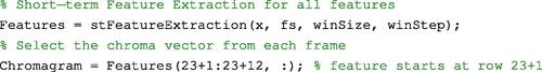
A large body of music thumbnailing techniques has adopted the Self-Similarity Matrix (SSM) of the recording as an intermediate signal representation [137]. This is also the case with the thumbnailing method that we are presenting here as a variant of the work in [31]. To compute the SSM of a music track, we first extract a sequence of short-term chroma vectors from the music recording, using the stFeatureExtraction() function that was introduced in Chapter 4.
To reduce the computational burden, we recommend that ![]() .
.
We then compute the pairwise similarity for every pair of vectors, ![]() , where
, where ![]() is the length of the feature sequence. The adopted similarity function is the correlation of the two vectors, defined as:
is the length of the feature sequence. The adopted similarity function is the correlation of the two vectors, defined as:

The resulting similarity values form the (![]() ) self-similarity matrix
) self-similarity matrix ![]() . Due to the fact that
. Due to the fact that ![]() , the SSM is symmetric with respect to its main diagonal, so we only need to focus on the upper triangle (where
, the SSM is symmetric with respect to its main diagonal, so we only need to focus on the upper triangle (where ![]() ) during the remaining steps of the thumbnailing scheme. Figure 8.1 presents the self-similarity matrix of a popular music track.
) during the remaining steps of the thumbnailing scheme. Figure 8.1 presents the self-similarity matrix of a popular music track.
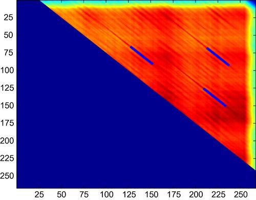
Figure 8.1 Self-similarity matrix for the track ‘True Faith’ by the band New Order. Detected thumbnails are shown with superimposed lines. For example, a pair of thumbnails occurs at segments with endpoints (in seconds) ![]() and
and ![]() . This corresponds to two repetitions of the the song’s chorus.
. This corresponds to two repetitions of the the song’s chorus.
The next processing stage bears its origins in the field of image analysis. Specifically, a diagonal mask is defined and applied as a moving average filter on the values of the SSM. The adopted mask is the ![]() identity matrix,
identity matrix, ![]() , where
, where ![]() is a user parameter that defines the desirable thumbnail length. By its definition, the mask has 1s on the main diagonal and 0s in all other elements. As an example, if the desirable thumbnail length is
is a user parameter that defines the desirable thumbnail length. By its definition, the mask has 1s on the main diagonal and 0s in all other elements. As an example, if the desirable thumbnail length is ![]() and the short-term processing step was previously set equal to
and the short-term processing step was previously set equal to ![]() , then
, then ![]() . Due to the fact that the mask is centered at each element of matrix
. Due to the fact that the mask is centered at each element of matrix ![]() , we prefer odd values for
, we prefer odd values for ![]() , so we would actually use
, so we would actually use ![]() in this case.
in this case.
The result of the moving average operation is a new matrix, ![]() , defined as
, defined as

After the masking operation has been completed, we find the highest value of matrix ![]() . If this value occurs at element
. If this value occurs at element ![]() , the respective pair of thumbnails consists of the feature sequences with indices
, the respective pair of thumbnails consists of the feature sequences with indices

In our implementation, the selection of highest value in matrix ![]() has been extended to cover (at most) the top three similarities. As a result, at most, three pairs of thumbnails will be extracted. In Figure 8.1, the detected pairs have been superimposed with lines on the SSM of the figure.
has been extended to cover (at most) the top three similarities. As a result, at most, three pairs of thumbnails will be extracted. In Figure 8.1, the detected pairs have been superimposed with lines on the SSM of the figure.
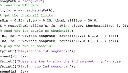
The musicThumbnailing() function implements our version of the music thumbnailing scheme. It returns the endpoints (in seconds) of one up to three pairs. The following MATLAB code demonstrates how to use the function for a music track that is stored in a WAVE file:
8.2 Music Meter and Tempo Induction
In this section, we present one more application of self-similarity analysis: a method that is capable of extracting the music meter and tempo of a music recording. The proposed scheme is a variant of the work in [138], which is based on the observation that the rhythmic characteristics of a music recording manifest themselves as inherent signal periodicities that can be extracted by processing the diagonals of the Self-Similarity Matrix (SSM).
The stages of the method are as follows:
1. The music signal is long-term segmented and the SSM of each long-term segment is generated. The short-term feature that we use is the set of standard MFCCs, although this is not a restrictive choice and the reader is encouraged to experiment with different sets of features. The Euclidean distance function is used to compute pairwise dissimilarities, so, strictly speaking, we are generating a dissimilarity matrix per long-term segment.
2. The mean value of each SSM diagonal is computed. A low mean value indicates a strong periodicity, with a period, measured in frames, equal to the index of the diagonal.
3. The sequence of mean values is treated as a signal, ![]() . An approximation,
. An approximation, ![]() , of the second derivative of this signal is computed and its maxima are detected.
, of the second derivative of this signal is computed and its maxima are detected.
4. The detected local maxima provide a measure of sharpness to the corresponding local minima of ![]() (signal periodicities).
(signal periodicities).
5. The local maxima are examined in pairs to determine if they fulfill certain criteria. The two main criteria are that the round-off error of the ratio of the indices of the respective diagonals should be as close to zero as possible (an appropriate threshold is used) and that the sum of heights of the peaks should be as high as possible. The best pair of local maxima, with respect to the selected criteria, is finally selected as the winner. The periodicities of the pair determine the tempo and music meter of the recording. If none of the pairs meets the criteria, the long-term segment returns a null value.
For the short-term feature extraction stage, recommended values for the length and step of the moving window are ![]() and
and ![]() , respectively. If each long-term segment is approximately
, respectively. If each long-term segment is approximately ![]() long,
long, ![]() vectors of MFCCs are generated from each long-term window and the dimensions of the resulting SSM are
vectors of MFCCs are generated from each long-term window and the dimensions of the resulting SSM are ![]() . This high computational load is due to the small hop size of the short-term window. However, this is the price we pay if we want to be able to measure the signal periodicities with sufficient accuracy.
. This high computational load is due to the small hop size of the short-term window. However, this is the price we pay if we want to be able to measure the signal periodicities with sufficient accuracy.
To compute an approximation, ![]() , of the second-order derivative of
, of the second-order derivative of ![]() , we first approximate the first-order derivative,
, we first approximate the first-order derivative, ![]() , and use the result to estimate the second-order derivative:
, and use the result to estimate the second-order derivative:
where ![]() is the maximum lag (diagonal index) for which
is the maximum lag (diagonal index) for which ![]() is computed. Assuming that, in popular music slow music meters can be up to
is computed. Assuming that, in popular music slow music meters can be up to ![]() long, the maximum lag,
long, the maximum lag, ![]() , for computing
, for computing ![]() is
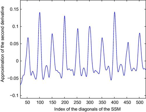
is ![]() . Figure 8.2 presents the first
. Figure 8.2 presents the first ![]() elements of sequence
elements of sequence ![]() for a
for a ![]() excerpt from a relatively fast Rumba dance taken from the Ballroom Dataset [131]. The three highest peaks occur at lags
excerpt from a relatively fast Rumba dance taken from the Ballroom Dataset [131]. The three highest peaks occur at lags ![]() , and
, and ![]() . The respective signal periodicities are
. The respective signal periodicities are ![]() , and
, and ![]() , which correspond to the durations of the beat
, which correspond to the durations of the beat ![]() , two beats
, two beats ![]() , and the music meter
, and the music meter ![]() .
.
After examining in pairs all peaks that exceed zero, the algorithm will eventually determine that the best pair of lags is ![]() . The equivalent of the first lag in beats per minute (bpm) is
. The equivalent of the first lag in beats per minute (bpm) is ![]() (bpm). Due to the fact that
(bpm). Due to the fact that ![]() and 120 bpm is a typical quarter-note duration in popular music, for this particular segment, the method will return that the beat is 120 bpm and that the music meter is
and 120 bpm is a typical quarter-note duration in popular music, for this particular segment, the method will return that the beat is 120 bpm and that the music meter is ![]() .
.
We provide an implementation of this algorithm in the musicMeterTempoInduction() function. To call this function, you first need to load a signal (e.g. from a WAVE file) and set values for the parameters of the method. Type:
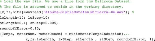
For a detailed explanation of the header of the function, type help musicMeterTempoInduction. If the last input argument is set to 1, the function prints its output on the screen. If you are interested in a very detailed scanning of the signal, set the long-term step, lwStep, equal to 1. Note that the implementation has not been optimized with respect to response times or memory consumption, so you are advised to experiment with relatively short music recordings, e.g. ![]() long.
long.
8.3 Music Content Visualization
Automatic, content-based visualization of large music collections can play an important, assisting role during the analysis of music content, because it can provide complementary representations of the music data. The goal of visualization systems is to analyze the audio content and represent a collection of music tracks in a 2D or 3D space, so that similar tracks are located closer to each other. In general, this can be achieved with dimensionality reduction methods which project the initial (high-dimensional) feature representation of the music data to low-dimensional spaces which can be easily visualized, while preserving the structure of the high-dimensional space. Dimensionality reduction approaches can be:
• Unsupervised: The dimensionality reduction of the feature space does not rely on prior knowledge, e.g. labeled data, because such information is unavailable.
• Supervised and semi-supervised: The techniques of this category exploit user-driven, prior knowledge of the problem at hand. For example, we may know track X is similar to track Y, so they have to be neighbors in the feature space, or that two feature vectors from the same music track have to be connected with a must-link constraint during a graph construction process.
In this section we provide brief descriptions of some widely used dimensionality reduction techniques that can be adopted in a content visualization context. In particular, we will present the methods of (a) random projection, (b) principal component analysis (PCA), (c) linear discriminant analysis, and (d) self-organizing maps. Other techniques that have been used for music content visualization are presented in [139], where multidimensional scaling (MDS) is adopted, and in [120], where the Isomap approach is used. Some of the methods have been left as exercises for the reader interested in delving deeper into the subject.
8.3.1 Generation of the Initial Feature Space
Before proceeding, let us first describe how to extract the initial feature space from a collection of music data based on the software library of this book. This can be achieved with function featureExtractionDir(), which extracts mid-term feature statistics for a list of WAVE files stored in a given folder. For example, type:
![]()
The function returns: (a) a cell array, where each cell contains a feature matrix, and (b) a cell array that contains the full path of each WAVE file of the input folder. Each element of the FeaturesDir cell array is a matrix of mid-term statistics that represents the respective music track. In order to represent the whole track using a single feature vector, this matrix is averaged over the mid-term vectors. This long-term averaging process is executed in functions musicVisualizationDemo() and musicVisualizationDemoSOM(), which are described later in this section. The reason that featureExtractionDir() does not return long-term averages (which are, after all, the final descriptors of each music track) but returns mid-term feature vectors instead, is that some of the visualization methods that will be described later use mid-term statistics to estimate the transformation that projects the long-term averages to the 2D subspace.
The featureExtractionDir() function is executed for two directories: (a) the first one is a collection of MP3 files (almost 300 in total) that cover a wide area of the pop-rock genre, and (b) the second one is a smaller collection of the same genre styles. The feature matrices, along with the song tiles, are stored in the musicLargeData.mat and musicSmallData.mat files. These are then used by the proposed visualization techniques.
8.3.2 Linear Dimensionality Reduction
We start with three basic linear dimensionality reduction approaches, one of which is supervised. These methods extract a lower dimensionality space as a continuous linear combination of the initial feature space, as opposed to the SOM approach (described in the next section), which operates in a discrete mode.
8.3.2.1 Random Projection
A straightforward solution to projecting a high-dimensional feature space to one of lower dimension, is by using a random matrix. Despite its simplicity, random projection has proved to be a useful technique, especially in the field of text retrieval, where the need to avoid excessive computational burden is of paramount importance [140]. Let ![]() data samples be arranged columnwise in matrix
data samples be arranged columnwise in matrix ![]() , where
, where ![]() is the dimensionality of the feature space. The projection to the space of lower dimension is defined as:
is the dimensionality of the feature space. The projection to the space of lower dimension is defined as:
where ![]() is the new dimension and
is the new dimension and ![]() is the random projection matrix. Equation (8.4) is also encountered in other linear projection methods; in the case of random projection,
is the random projection matrix. Equation (8.4) is also encountered in other linear projection methods; in the case of random projection, ![]() is randomly generated. Note, that before applying random projection, a feature normalization step (to zero mean and unity standard deviation) is required, in order to remove the bias due to features with higher values.
is randomly generated. Note, that before applying random projection, a feature normalization step (to zero mean and unity standard deviation) is required, in order to remove the bias due to features with higher values.
8.3.2.2 Principal Component Analysis
Principal component analysis (PCA) is a widely adopted dimensionality reduction method aimed at reducing the dimensionality of the feature space while preserving as much ‘data variance’ (of the initial space) as possible [141,142]. In general, PCA computes the eigenvalue decomposition of an estimate of the covariance matrix of the data and uses the most important eigenvectors to project the feature space to a space of lower dimension. In other words, the physical meaning of the functionality of the PCA method is that it projects to a subspace that maintains most of the variability of the data.
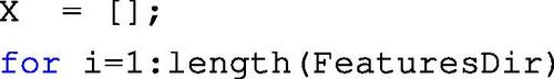
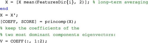
PCA is implemented in the princomp() function of MATLAB’s Statistics Toolbox. princomp(), accepts one single input argument, the feature matrix, and returns a matrix with the principal components. The first ![]() columns of that matrix, which stand for the most dominant components, are used to project the initial feature space to the reduced
columns of that matrix, which stand for the most dominant components, are used to project the initial feature space to the reduced ![]() -dimensional space. From an implementation perspective, if FeaturesDir() is the cell array of mid-term feature statistics (output of featureExtractionDir()), then the PCA projection matrix is generated as follows:
-dimensional space. From an implementation perspective, if FeaturesDir() is the cell array of mid-term feature statistics (output of featureExtractionDir()), then the PCA projection matrix is generated as follows:
8.3.2.3 Fisher Linear Discriminant Analysis
PCA is an unsupervised method; it seeks a linear projection that preserves the variance of the samples, without using class information. However, we are often interested in maintaining the association among features and class labels, when such information is available. The Fisher linear discriminant analysis method (FLD, also known as LDA) is another linear dimensionality reduction technique that exploits the idea of embedding supervised knowledge in the procedure. This means that, in order to compute the projection matrix, we need to know the mappings of feature vectors in the initial feature space to predefined class labels. The basic idea behind LDA is that, in the lower-dimensional space, the centroids of the classes must be far from each other, while the variance within each class must be small [143]. Therefore, LDA seeks the subspace that maximizes discrimination among classes, whereas PCA seeks the subspace that preserves most the variance among the feature vectors.
The FLD method is not included in MATLAB. We have selected the fld() function, which is available on the Mathworks File Exchange website.1 This function accepts the following arguments: a ![]() feature matrix, a
feature matrix, a ![]() label matrix and the desired number of dimensions,
label matrix and the desired number of dimensions, ![]() . It returns the optimal Fisher orthonormal matrix (
. It returns the optimal Fisher orthonormal matrix (![]() ), which is used to project the initial feature set to the new dimensionality.
), which is used to project the initial feature set to the new dimensionality.
The obvious problem with the FLD approach, in the context of a data visualization application, is that it needs supervised knowledge to function properly. So, the question is how we can obtain mappings of feature vectors to class labels. We adopt the following rationale to solve this problem:
In this way, the FLD method will try to generate a linear transform of the original data that minimizes the variance between the feature vectors (mid-term statistics) of the same class (music track), while maximizing the distances between the means of the classes. This trick enables us to feed the FLD algorithm with a type of supervised knowledge that stems from the fact that feature vectors from the same musical track must share the same class label. The extracted orthonormal matrix is used to project the long-term averaged feature statistics (one long-term feature vector for each music track). The following code demonstrates how to generate the FLD orthonormal matrix using the steps described above (again, FeaturesDir is a cell array of mid-term feature statistics):

8.3.2.4 Visualization Examples
The three linear dimensionality reduction approaches that were described above (random projection, PCA, and LDA) have been implemented in the musicVisualizationDemo() function of the library. The function takes as input (a) the cell array of feature matrices, (b) the cell array of WAVE file paths, and (c) which dimensionality reduction method to use (0 for random projection, 1 for PCA, and 2 for LDA). The first two arguments are generated by featureExtractionDir(), as described in the beginning of Section 8.3.
We have demonstrated the results of the linear dimensionality reduction methods using the dataset stored in the musicSmallData.mat file, because the content of the large dataset would be a lot harder to illustrate. The musicSmallData.mat dataset is a subset of the larger one and consists of 40 audio tracks from 4 different artists. Two of the artists can be labeled as punk rock Bad Religion and NOFX and the other two as Synthpop (New Order and Depeche Mode). The code that performs the visualization of this dataset using all three methods (random projection, PCA, and LDA) is as follows:
Figure 8.3 shows the visualization results for all three linear projection methods. It can be seen that the LDA-generated visualization achieves higher discrimination between artists and genres (the songs of New Order are on the same plane as the Depeche Mode tracks). The random projection method confuses dissimilar tracks in many cases.

Figure 8.3 Visualization results for the three linear dimensionality reduction approaches, applied on the musicSmallData.mat dataset. Note that the length of the track titles has been truncated for the sake of clarity.
8.3.3 Self-Organizing Maps
Self-Organizing Maps (SOMs) provide a useful approach to data visualization. They are capable of generating 2D quantized (discretized) representations of an initial feature space [114–116]. SOMs are neural networks trained in an unsupervised mode in order to produce the desired data organizing map [144]. An important difference among SOMs and typical neural networks is that each node (neuron) of a SOM has a specific position in a defined topology of nodes. In other words, SOMs implement a projection of the initial high-dimensional feature space to a lower-dimensional grid of nodes (neurons).
In MATLAB, SOMs have been implemented in the Neural Network Toolbox. To map a feature space to a 2D SOM, we need to use the selforgmap(), train(), and net() functions. The following code demonstrates how this is achieved, given a matrix, X, that contains the vectors of the initial feature space:

Parameter nGrid stands for the dimensions of the grid of neurons (![]() ). Variable classes contain the class label for each input sample. Note that the example adopted the gridtop topology, so class label 1 corresponds to the neuron at position (0,0), class label 2 to position (1,0), and so on. The gridtop topology of the SOM is shown in Figure 8.4, which is for a
). Variable classes contain the class label for each input sample. Note that the example adopted the gridtop topology, so class label 1 corresponds to the neuron at position (0,0), class label 2 to position (1,0), and so on. The gridtop topology of the SOM is shown in Figure 8.4, which is for a ![]() grid. Other MATLAB-supported grids are the hextop and randtop topologies.
grid. Other MATLAB-supported grids are the hextop and randtop topologies.
Function musicVisualizationDemoSOM() demonstrates how to use SOMs to map a high-dimensional space of audio features to a 2D plane. Note that the first two input arguments of this function are similar to the arguments of the musicVisualizationDemo() function. The third input argument is the size of the grid and the fourth is the type of method: 0 for direct SOM dimensionality reduction and 1 for executing the LDA as a preprocessing step.2 Overall, the musicVisualizationDemoSOM() function maps each feature vector of the initial feature space to a node (neuron) of the SOM grid. In the end of the training phase, each node of the grid contains a set of music tracks. The number of tracks that have been assigned to each node is plotted in the respective area of the grid and when the user clicks on a node, the respective music track titles are visualized in a separate plotting area (see Figure 8.5).

Figure 8.5 Visualization of selected nodes of the SOM of the data in the musicLargeData.mat dataset.
We have used the audio features in the musicLargeData.mat file to demonstrate the functionality of the SOM-based music content representation. The following lines of MATLAB code visualize the dataset stored in the musicLargeData.mat file using the SOM scheme:
![]()
The grid size for this example is ![]() . Figure 8.5 presents some node visualization examples. It can be seen that in some cases, the music tracks that were assigned to the same node of the grid share certain common characteristics. For example, the first example contains songs with female vocalists. The rest of the examples mostly highlight songs of the same artist. In some cases, the proximity of two nodes has a physical meaning: the 3rd and the 4th examples are (practically) homogeneous with respect to the identity of the artist, and in addition, the two artists can be considered to belong to similar musical genres (Green Day and Bad Religion both fall into the punk-rock genre).
. Figure 8.5 presents some node visualization examples. It can be seen that in some cases, the music tracks that were assigned to the same node of the grid share certain common characteristics. For example, the first example contains songs with female vocalists. The rest of the examples mostly highlight songs of the same artist. In some cases, the proximity of two nodes has a physical meaning: the 3rd and the 4th examples are (practically) homogeneous with respect to the identity of the artist, and in addition, the two artists can be considered to belong to similar musical genres (Green Day and Bad Religion both fall into the punk-rock genre).
8.4 Exercises
1. (D5) Section 8.3 presented various content visualization techniques. One of those approaches, the LDA dimensionality reduction method, requires the use of a set of class labels (one class label per music track) to operate. In a way, the generated labels do not actually indicate classes, but simply discriminate between different music tracks. In this exercise you are asked to extend the functionality of musicVisualizationDemo(), by making use of human annotations as follows:
• The user is prompted with an initial visualization of the music content, generated by the LDA approach (function musicVisualizationDemo()).
• The user manually selects a set of similar musical tracks. The selection starts and ends with a right click of the mouse. The user uses the left mouse button to select a set of similar tracks and the respective track IDs are stored.
• The visualization of the content is repeated with the LDA approach. However, this time, the class labels used in the LDA algorithm are “enchanched” by the user’s selections: the set of selected musical tracks is given the same class label. In other words, the user provides some supervised information based on his/her perception of music similarity.
• Steps 2 and 3 are repeated a predefined number of times.
In this way, we expect that the resulting two-dimensional visualization will be adapted to the user’s perception of the dataset.
2. (D3) Function musicVisualizationDemo() computes a projection matrix for each one of the adopted linear dimensionality reduction approaches (random projection, PCA, and LDA). As described in Section 8.3, for the first two methods (random projection and PCA) the long-term averages of the feature statistics of each music track are used, whereas LDA uses the mid-term feature vectors of each track. Change the code of musicVisualizationDemo() so that random projection and PCA also use the mid-term feature vectors, instead of their averages. Can you see any differences in the resulting visualization results? Justify your answer. Use the musicSmallData.mat training. Note: In all cases, the final representation is based on the projection of long-term averages; what we ask here is to compute the projection transform based on the mid-term features.
3. (D4) Multidimensional scaling (MDS) is yet another widely used technique for data visualization, which has also been used in music information retrieval applications [139]. It focuses on representing the (dis)similarities amongst samples of a dataset, by means of a distance matrix. In MATLAB, MDS is implemented in the mdscale() function of the Statistics Toolbox. Apply mdscale() on the musicSmallData.mat dataset to visualize the respective music tracks in the 2D space. For more information on the mdscale() function, you may need to read the respective online MATLAB documentation.3 Hint 1: You first need to perform feature normalization on the initial dataset (zero mean and unity standard deviation). Hint 2: Use pdist() to compute a distance matrix between the feature vectors of the dataset.
4. (D5) The Isomap method has also been used to visualize music content [120]. The Isomap algorithm [145] is actually a non-linear extension of the multidimensional scaling (MDS) method. Use the MATLAB implementation of the Isomap algorithm in http://isomap.stanford.edu/![]() to visualize the dataset stored in the musicSmallData.mat file. Note that the Isomap() function expects a distance matrix as an input argument (you will need to carefully read the documentation before you proceed). Hint: You first need to perform feature normalization (to zero mean and unity standard deviation) on the initial dataset.
to visualize the dataset stored in the musicSmallData.mat file. Note that the Isomap() function expects a distance matrix as an input argument (you will need to carefully read the documentation before you proceed). Hint: You first need to perform feature normalization (to zero mean and unity standard deviation) on the initial dataset.
5. (D3) In this exercise the reader is encouraged to experiment with all visualization approaches described in Section 8.3, using their own music data. To this end, you must first perform feature extraction on a directory of music data using the featureExtractionDir() function.
6. (D4) The SOM-based visualization approach (Section 8.3.3) leads to a discretized representation of the final 2D space, which means that usually more than one sample (in our case, music tracks) will be mapped to a single SOM node. Combine the SOM and LDA approaches for the purposes of music content visualization. The core of the new visualization function must be the SOM approach. However, when the user selects a particular SOM grid node, instead of simply printing the respective song titles (as happens in musicVisualizationDemoSOM()), your function must use the LDA dimensionality reduction approach to plot the respective song titles in the 2D space. Obviously, the LDA algorithm must be trained on the samples that are mapped to the selected SOM grid (and not on the whole dataset).
7. (D5) Implement a query-by-humming system that broadly speaking, follows the guidelines of the MIREX 2011 Query-by-Singing/Humming contest http://www.music-ir.org/mirex/wiki/2011:Query-by-Singing/Humming_Results#Task_Descriptions![]() . The following steps outline the tasks that you need to complete:
. The following steps outline the tasks that you need to complete:
(a) Download Roger Jang’s MIR-QBSH corpus from http://mirlab.org/dataSet/public/MIR-QBSH-corpus.rar![]() . This consists of the sung tunes of 48 tracks. The sung melodies are organized in folders based on the year of recording and the singer. The name of each WAVE file reveals the melody to which it refers. Each audio file is accompanied by an extracted pitch sequence.
. This consists of the sung tunes of 48 tracks. The sung melodies are organized in folders based on the year of recording and the singer. The name of each WAVE file reveals the melody to which it refers. Each audio file is accompanied by an extracted pitch sequence.
(b) Place all audio and pitch files in a single folder. To avoid duplicate file names, use a script to rename each file so that the recording year and the person’s id become part of the string of the file name.
(c) Match each pitch sequence against all others using the Itakura local path constraints. Sort the matching costs in ascending order and examine the best 10 results. If the majority of results stem from the same melody, a success is recorded.
(d) Repeat the previous step for all pitch sequences and compute the accuracy of the system.
In a way, we are using a version of the leave-one-out method for performance validation. Repeat with the Sakoe local-path constraints and the Smith-Waterman algorithm. For the latter, you will need to devise a modified similarity function (why?). Finally, experiment with endpoint constraints (see also the related exercises in Chapter 7).
8. (D5) Develop a MATLAB function that converts a WAVE file to a sequence of notes. It is assumed that we are dealing with monophonic recordings of a single instrument. Your function will need to perform the following tasks:
(a) Load the WAVE file.
(b) Perform pitch tracking (see also Chapter 4).
(c) Quantize each value of the pitch sequence to the closest semitone of the chromatic scale.
(d) Convert the sequence of quantized pitch values to a sequence of vectors of the form ![]() where
where ![]() is the pitch value and
is the pitch value and ![]() is its duration (you will need to merge successive pitch values to a single vector if they are equal).
is its duration (you will need to merge successive pitch values to a single vector if they are equal).
(e) Drop short notes. Any note with a duration shorter than a user-defined threshold is eliminated.
(f) The remaining sequence of vectors is stored in a text file.
In addition, develop a second function that loads the previously generated text file, converts it to the MIDI format, and uses an external MIDI player to playback the result. You may need to download a 3d-party, publicly available MATLAB toolbox to implement the MIDI functionality. Alternatively, you can reproduce the stored file as a sequence of simple tones. The result might not please the ear but it will give you an idea of how successful your music transcription function has been.
1 Mathworks File Exchange, Fischer Linear Dicriminant Analysis, by Sergios Petridis: http://www.mathworks.com/matlabcentral/fileexchange/38950-fischer-linear-dicriminant-analysis![]() .
.
2 We have selected to use LDA as a preprocessing step. The LDA method is first employed to reduce the dimensionality of the feature space to 10 dimensions and the SOM is then trained on a 10-dimensional feature space. In this way, the training time of the SOM is reduced significantly.