
Stochastic Returns and Risk
Now allow for risk and uncertainty (strictly speaking, these are different concepts—see the discussion in Chapter 11). We could think of returns as being random, or stochastic, but it is more intuitively appealing to model returns as being state dependent. For example, suppose the dollar payoff to asset j, Xj, depends on which state of nature is observed. Assume there are six such states and the payoff will be one of the following ![]() , all with likelihood
, all with likelihood ![]() . Clearly, the payoff (and return) to Xj is random with uniform distribution in this case. We are interested in estimating the expected payoff, which, to us, is the mean value of Xj across all states. In general, the expected value E(Xj) is a weighted average of the possible outcomes. Formally, this is
. Clearly, the payoff (and return) to Xj is random with uniform distribution in this case. We are interested in estimating the expected payoff, which, to us, is the mean value of Xj across all states. In general, the expected value E(Xj) is a weighted average of the possible outcomes. Formally, this is ![]() ; where Xi is a state value and f(xi) denotes the probability of that state being realized; here,
; where Xi is a state value and f(xi) denotes the probability of that state being realized; here, ![]() for all i outcomes. That is:
for all i outcomes. That is:
![]()
So, the expected payoff is 1.5. This statistic conveys a notion of average value across all states. That is, if we were to keep track of our payoffs over time, averaging them as we go along, that average would approach 1.5 by the central limit theorem.
Because the realized payoff is not known with certainty, an investment in X is risky. Although the expected payoff is constant at ![]() , the observed payoff will vary, being as high as 4 and as low as –1. Translating payoffs into returns is simple—if we have an initial investment $X0 = say, $1, then the return is the percentage change in value upon realizing the payoff, for example, if
, the observed payoff will vary, being as high as 4 and as low as –1. Translating payoffs into returns is simple—if we have an initial investment $X0 = say, $1, then the return is the percentage change in value upon realizing the payoff, for example, if ![]() , then the return is 100 percent.
, then the return is 100 percent.
Risk is captured in the variability of payoffs. See Appendix 5.1 for a review of statistics. Variance is defined as:
![]()
This is also a weighted sum—in this case, a weighted sum of squared deviations from the mean:
![]()
The square root of 2.92 is 1.71, which is the standard deviation—what financial analysts refer to as volatility. We can summarize our stochastic world of payoffs as having an expected payoff of 1.5 and a standard deviation of 1.71 around this mean. Payoffs, and therefore, returns, have a central tendency (the mean) and dispersion (the volatility) that captures our notion of risk. Risk increases with volatility.
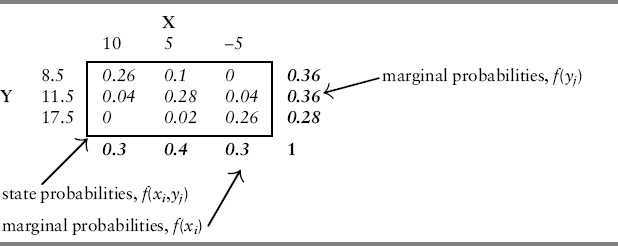
Let's expand this thinking to two assets, X and Y, but with their returns state dependent. A portfolio of X and Y will have variance that is the sum of the variance of X and the variance of Y plus two times their covariance. To illustrate, consider Figure 5.1, which depicts returns for assets X and Y in three possible states. State probabilities are given in the interior of the table and correspond to the likelihood of joint returns (for example, the probability that X returns 10 and Y returns 8.5 occurs 26 percent of the time). The probability that X's outcome is 10 is called the marginal probability for X and is 0.3, or 30 percent. Similar thinking holds for Y. For example, the marginal probability for Y returning 8.5 is 0.36 and so on. Thus, the marginal probability of ![]() is the likelihood that Y will have this outcome regardless of what outcome X has jointly; it is
is the likelihood that Y will have this outcome regardless of what outcome X has jointly; it is ![]() . The | operator denotes a conditional probability.
. The | operator denotes a conditional probability.
Figure 5.1 State Contingent Claims
Let's estimate the following statistics (see also Chapter 5 Examples.xlsx):
![]()
![]()
![]()
The reader should confirm the statistics ![]()
![]() .
.
We also note that X and Y are obviously not independent—independence would imply their joint probabilities to be zero. That means the covariation between these two random variables is nonzero. We denote this covariance by Cov(X,Y) and define it as:
![]()
Again, this is an expected value and it is therefore a weighted sum of the products. This expression can be simplified since (see Appendix 5.1):
![]()
and where ![]() and
and ![]() .
.
Therefore, ![]() and
and ![]()
![]() .
.
Referring to Figure 5.1 again, we see that this is a double summation because we must sum over X (or Y) first, and then the other term Y (or X). Doing that gives us
![]()
It is a negative number because the payoffs for Y tend to be high when those for X are low. You can see this from the tabled data; for example, when Y has its highest payoff at 17.5, X has its lowest payoff at –5. Thus, these two payoffs are negatively correlated. That's an attractive property that we will address shortly.
Correlation is a standardized covariance. Standardization places the correlation coefficient ρ in the interval, ![]() . The correlation coefficient itself is just the covariance between X and Y divided by the product of their standard deviations. Thus,
. The correlation coefficient itself is just the covariance between X and Y divided by the product of their standard deviations. Thus,
![]()
You should confirm for the data in the preceding table that ![]() .
.
To make the intuition a little easier, recall that any random variable's covariance with itself is the same as its variance, that is, ![]()
![]() . Covariance is critical to understanding and managing portfolio risk and forms the basis of asset allocation and risk diversification, as we shall see shortly.
. Covariance is critical to understanding and managing portfolio risk and forms the basis of asset allocation and risk diversification, as we shall see shortly.
Suppose we form a portfolio on X and Y in which X has weight w and Y has weight ![]() so that the portfolio is fully invested, that is, the weights sum to one. Then the return to this portfolio, r, is:
so that the portfolio is fully invested, that is, the weights sum to one. Then the return to this portfolio, r, is:
![]()
The expected return on the portfolio is therefore:
![]()
The expected portfolio return therefore depends on what proportion of each asset is held in the portfolio. The risk on the portfolio will depend on the individual risks to assets X and Y as well as the degree to which the returns on these two assets covary. The variance of the portfolio return is defined as:
![]()
Expanding the square and taking expectations yields:
![]()
More simply,
![]()
Here, ![]() is the covariance. Since returns are expressed in percent and variance in percent squared, taking the square root converts risk back to percent; hence, we typically refer to the risk on the portfolio as its percent volatility, or standard deviation, σ.
is the covariance. Since returns are expressed in percent and variance in percent squared, taking the square root converts risk back to percent; hence, we typically refer to the risk on the portfolio as its percent volatility, or standard deviation, σ.
We will find it useful later to use the definition of the correlation and write the portfolio variance as follows:
![]()
Notice that as the correlation between the two asset returns moves from +1 towards –1, portfolio risk declines.
Let's generalize to N assets in a portfolio again, each of which has random return ri. Suppose we know the individual expected returns on the assets in the portfolio as E(ri) for ![]() . The return on the portfolio is:
. The return on the portfolio is: ![]() and has expected return (mean) equal to:
and has expected return (mean) equal to:
![]()
The expected return on the portfolio is the weighted sum of the expected returns on the individual assets in the portfolio.
The variance of the portfolio is therefore defined as:
![]()
Notice that this is a quadratic form (it involves a sum of squares). The weights wi take the place of the probability weights f(xi) in our state contingent claims example while the ![]() replace the means μx and so forth. When
replace the means μx and so forth. When ![]() , we are then looking at the variance. Otherwise, we are estimating the covariances between returns on different assets. An equivalent expression is:
, we are then looking at the variance. Otherwise, we are estimating the covariances between returns on different assets. An equivalent expression is:
![]()
which, after passing the expectations operator past the sum of the product of the weights (these are constants, remember, and the expectation of a constant times a random variable is the constant times the expectation of the random variable). Therefore, the expectations of the product of the deviations of the returns from their means are the covariances (variances if ![]() ), which is:
), which is:
![]()
Note that ![]() ; for
; for ![]() .
.