
Discriminant Analysis Overview
Discriminant analysis attempts to classify observations described by values on continuous variables into groups. Group membership, defined by a categorical variable X, is predicted by the continuous variables. These variables are called covariates and are denoted by Y.
Discriminant analysis differs from logistic regression. In logistic regression, the classification variable is random and predicted by the continuous variables. In discriminant analysis, the classifications are fixed, and the covariates (Y) are realizations of random variables. However, in both techniques, the categorical value is predicted by the continuous variables.
The Discriminant platform provides four methods for fitting models. All methods estimate the distance from each observation to each group's multivariate mean (centroid) using Mahalanobis distance. You can specify prior probabilities of group membership and these are accounted for in the distance calculation. Observations are classified into the closest group.
Fitting methods include the following:
• Linear—Assumes that the within-group covariance matrices are equal. The covariate means for the groups defined by X are assumed to differ.
• Quadratic—Assumes that the within-group covariance matrices differ. This requires estimating more parameters than does the Linear method. If group sample sizes are small, you risk obtaining unstable estimates.
• Regularized—Provides two ways to impose stability on estimates when the within-group covariance matrices differ. This is a useful option if group sample sizes are small.
• Wide Linear—Useful in fitting models based on a large number of covariates, where other methods can have computational difficulties. It assumes that all covariance matrices are equal.
Example of Discriminant Analysis
In Fisher's Iris data set, four measurements are taken from a sample of Iris flowers consisting of three different species. The goal is to identify the species accurately using the values of the four measurements.
1. Select Help > Sample Data Library and open Iris.jmp.
2. Select Analyze > Multivariate Methods > Discriminant.
3. Select Sepal length, Sepal width, Petal length, and Petal width and click Y, Covariates.
4. Select Species and click X, Categories.
5. Click OK.
Figure 5.2 Discriminant Analysis Report Window
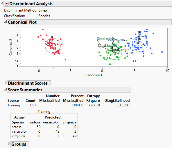
Because there are three classes for Species, there are two canonical variables. In the Canonical Plot, each observation is plotted against the two canonical coordinates. The plot shows that these two coordinates separate the three species. Since there was no validation set, the Score Summaries report shows a panel for the Training set only. When there is no validation set, the entire data set is considered the Training set. Of the 150 observations, only three are misclassified.
Discriminant Launch Window
Launch the Discriminant platform by selecting Analyze > Multivariate Methods > Discriminant.
Figure 5.3 Discriminant Launch Window for Iris.jmp

Note: The Validation button appears in JMP Pro only. In JMP, you can define a validation set using excluded rows. See “Validation in JMP and JMP Pro”.
Y, Covariates
Columns containing the continuous variables used to classify observations into categories.
X, Categories
A column containing the categories or groups into which observations are to be classified.
Weight
A column whose values assign a weight to each row for the analysis.
Freq
A column whose values assign a frequency to each row for the analysis. In general terms, the effect of a frequency column is to expand the data table, so that any row with integer frequency k is expanded to k rows. You can specify fractional frequencies.
A numeric column containing two or three distinct values:
‒ If there are two values, the smaller value defines the training set and the larger value defines the validation set.
‒ If there are three values, these values define the training, validation, and test sets in order of increasing size.
‒ If there are more than three values, all but the smallest three are ignored.
If you click the Validation button with no columns selected in the Select Columns list, you can add a validation column to your data table. For more information about the Make Validation Column utility, see the Modeling Utilities chapter in the Predictive and Specialized Modeling book.
By
Performs a separate analysis for each level of the specified column.
Stepwise Variable Selection
Performs stepwise variable selection using covariance analysis and p-values. For details, see “Stepwise Variable Selection”.
If you have specified a validation set, statistics that have been calculated for the validation set appear.
Note: This option is not provided for the Wide Linear discriminant method.
Discriminant Method
Provides four methods for conducting discriminant analysis. See “Discriminant Methods”.
Shrink Covariances
Shrinks the off-diagonal entries of the pooled within-group covariance matrix and the within-group covariance matrices. See “Shrink Covariances”.
Uncentered Canonical
Suppresses centering of canonical scores for compatibility with older versions of JMP.
Use Pseudoinverses
Uses Moore-Penrose pseudoinverses in the analysis when the covariance matrix is singular. The resulting scores involve all covariates. If left unchecked, the analysis drops covariates that are linear combinations of covariates that precede them in the list of Y, Covariates.
Stepwise Variable Selection
Note: Stepwise Variable Selection is not available for the Wide Linear method.
If you select the Stepwise Variable Selection option in the launch window, the Discriminant Analysis report opens, showing the Column Selection panel. Perform stepwise analysis, using the buttons to select variables or selecting them manually with the Lock and Entered check boxes. Based on your selection F ratios and p-values are updated. For details about how these are updated, see “Updating the F Ratio and Prob>F”.
Figure 5.4 Column Selection Panel for Iris.jmp with a Validation Set

Note: The Go button only appears when you use excluded rows for validation in JMP or a validation column in JMP Pro.
Updating the F Ratio and Prob>F
When you enter or remove variables from the model, the F Ratio and Prob>F values are updated based on an analysis of covariance model with the following structure:
• The covariate under consideration is the response.
• The covariates already entered into the model are predictors.
• The group variable is a predictor.
The values for F Ratio and Prob>F given in the Stepwise report are the F ratio and p-value for the analysis of covariance test for the group variable. The analysis of covariance test for the group variable is an indicator of its discriminatory power relative to the covariate under consideration.
Statistics
Columns In
Number of columns currently selected for entry into the discriminant model.
Columns Out
Number of columns currently available for entry into the discriminant model.
Smallest P to Enter
Smallest p-value among the p-values for all covariates available to enter the model.
Largest P to Remove
Largest p-value among the p-values for all covariates currently selected for entry into the model.
Validation Entropy RSquare
Entropy RSquare for the validation set. Larger values indicate better fit. An Entropy RSquare value of 1 indicates that the classifications are perfectly predicted. Because uncertainty in the predicted probabilities is typical for discriminant models, Entropy RSquare values tend to be small.
See “Entropy RSquare”. Available only if a validation set is used.
Note: It is possible for the Validation Entropy RSquare to be negative.
Validation Misclassification Rate
Misclassification rate for the validation set. Smaller values indicate better classification. Available only if a validation set is used.
Buttons
Step Forward
Enters the most significant covariate from the covariates not yet entered. If a validation set is used, the Prob>F values are based on the training set.
Step Backward
Removes the least significant covariate from the covariates entered but not locked. If a validation set is used, Prob>F values are based on the training set.
Enter All
Enters all covariates by checking all covariates that are not locked in the Entered column.
Remove All
Removes all covariates that are not locked by deselecting them in the Entered column.
Apply this Model
Produces a discriminant analysis report based on the covariates that are checked in the Entered columns. The Select Columns outline is closed and the Discriminant Analysis window is updated to show analysis results based on your selected Discriminant Method.
Tip: After you click Apply this Model, the columns that you select appear at the top of the Score Summaries report.
Go
Enters covariates in forward steps until the Validation Entropy RSquare begins to decrease. Entry terminates when two forward steps are taken without improving the Validation Entropy RSquare. Available only with excluded rows in JMP or a validation column in JMP Pro.
Columns
Lock
Forces a covariate to stay in its current state regardless of any stepping using the buttons.
Note the following:
‒ If you enter a covariate and then select Lock for that covariate, it remains in the model regardless of selections made using the control buttons. The Entered box for the locked covariate shows a dimmed check mark to indicate that it is in the model.
‒ If you select Lock for a covariate that is not Entered, it is not entered into the model regardless of selections made using the control buttons.
Entered
Indicates which columns are currently in the model. You can manually select columns in or out of the model. A dimmed check mark indicates a locked covariate that has been entered into the model.
Column
Covariate of interest.
F Ratio
F ratio for a test for the group variable obtained using an analysis of covariance model. For details, see “Updating the F Ratio and Prob>F”.
Prob > F
p-value for a test for the group variable obtained using an analysis of covariance model. For details, see “Updating the F Ratio and Prob>F”.
Stepwise Example
For an illustration of how to use Stepwise, consider the Iris.jmp sample data table.
1. Select Help > Sample Data Library and open Iris.jmp.
2. Select Analyze > Multivariate Methods > Discriminant.
3. Select Sepal length, Sepal width, Petal length, and Petal width and click Y, Covariates.
4. Select Species and click X, Categories.
5. Select Stepwise Variable Selection.
6. Click OK.
7. Click Step Forward three times.
Three covariates are entered into the model. The Smallest P to Enter appears in the top panel. It is 0.0103288, indicating that the remaining covariate, Sepal length, might also be valuable in a discriminant analysis model for Species.
Figure 5.5 Stepped Model for Iris.jmp

8. Click Apply This Model.
The Column Selection outline is closed. The window is updated to show reports for a fit based on the entered covariates and your selected discriminant method.
Note that the covariates that you selected for your model are listed at the top of the Score Summaries report.
Figure 5.6 Score Summaries Report Showing Selected Covariates

Discriminant Methods
JMP offers these methods for conducting Discriminant Analysis: Linear, Quadratic, Regularized, and Wide Linear. The first three methods differ in terms of the underlying model. The Wide Linear method is an efficient way to fit a Linear model when the number of covariates is large.
Note: When you enter more than 500 covariates, a JMP Alert recommends that you switch to the Wide Linear method. This is because computation time can be considerable when you use the other methods with a large number of columns. Click Wide Linear, Many Columns to switch to the Wide Linear method. Click Continue to use the method you originally selected.
Figure 5.7 Linear, Quadratic, and Regularized Discriminant Analysis

The Linear, Quadratic, and Regularized methods are illustrated in Figure 5.7. The methods are described here briefly. For technical details, see “Saved Formulas”.
Linear, Common Covariance
Performs linear discriminant analysis. This method assumes that the within-group covariance matrices are equal. See“Linear Discriminant Method”.
Quadratic, Different Covariances
Performs quadratic discriminant analysis. This method assumes that the within-group covariance matrices differ. This method requires estimating more parameters than the Linear method requires. If group sample sizes are small, you risk obtaining unstable estimates. See “Quadratic Discriminant Method”.
If a covariate is constant across a level of the X variable, then its related entries in the within-group covariance matrix have zero covariances. To enable matrix inversion, the zero covariances are replaced with the corresponding pooled within covariances. When this is done, a note appears in the report window identifying the problematic covariate and level of X.
Tip: A shortcoming of the quadratic method surfaces in small data sets. It can be difficult to construct invertible and stable covariance matrices. The Regularized method ameliorates these problems, still allowing for differences among groups.
Regularized, Compromise Method
Provides two ways to impose stability on estimates when the within-group covariance matrices differ. This is a useful option when group sample sizes are small. See “Regularized, Compromise Method” and “Regularized Discriminant Method”.
Wide Linear, Many Columns
Useful in fitting models based on a large number of covariates, where other methods can have computational difficulties. This method assumes that all within-group covariance matrices are equal. This method uses a singular value decomposition approach to compute the inverse of the pooled within-group covariance matrix. See “Description of the Wide Linear Algorithm”.
Note: When you use the Wide Linear option, a few of the features that normally appear for other discriminant methods are not available. This is because the algorithm does not explicitly calculate the very large pooled within-group covariance matrix.
Regularized, Compromise Method
Regularized discriminant analysis is governed by two nonnegative parameters.
• The first parameter (Lambda, Shrinkage to Common Covariance) specifies how to mix the individual and group covariance matrices. For this parameter, 1 corresponds to Linear Discriminant Analysis and 0 corresponds to Quadratic Discriminant Analysis.
• The second parameter (Gamma, Shrinkage to Diagonal) is a multiplier that specifies how much deflation to apply to the non-diagonal elements (the covariances across variables). If you choose 1, then the covariance matrix is forced to be diagonal.
Assigning 0 to each of these two parameters is identical to requesting quadratic discriminant analysis. Similarly, assigning 1 to Lambda and 0 to Gamma requests linear discriminant analysis. Use Table 5.1 to help you decide on the regularization. See Figure 5.7 for examples of linear, quadratic, and regularized discriminant analysis.
|
Use Smaller Lambda
|
Use Larger Lambda
|
Use Smaller Gamma
|
Use Larger Gamma
|
|
Covariance matrices differ
|
Covariance matrices are identical
|
Variables are correlated
|
Variables are uncorrelated
|
|
Many rows
|
Few rows
|
|
|
|
Few variables
|
Many variables
|
|
|
Shrink Covariances
In the Discriminant launch window, you can select the option to Shrink Covariances. This option is recommended when some groups have a small number of observations. Discriminant analysis requires inversion of the covariance matrices. Shrinking off-diagonal entries improves their stability and reduces prediction variance. The Shrink Covariances option shrinks the off-diagonal entries by a factor that is determined using the method described in Schafer and Strimmer, 2005.
If you select the Shrink Covariances option with the Linear discriminant method in the launch window, this provides a shrinkage of the covariance matrices that is equivalent to the shrinkage provided by the Regularized discriminant method with appropriate Lambda and Gamma values. When you select the Shrink Covariances option and run your analysis, the Shrinkage report gives you an Overall Shrinkage value and an Overall Lambda value. To obtain the same analysis using the Regularized method, enter 1 as Lambda and the Overall Lambda from the Shrinkage report as Gamma in the Regularization Parameters window.
The Discriminant Analysis Report
The Discriminant Analysis report provides discriminant results based on your selected Discriminant Method. The Discriminant Method and the Classification variable are shown at the top of the report. If you selected the Regularized method, its associated parameters are also shown.
You can change Discriminant Method by selecting the option from the red triangle menu. The results in the report update to reflect the selected method.
Figure 5.8 Example of a Discriminant Analysis Report
The default Discriminant Analysis report is shown in Figure 5.8 and contains the following sections:
• When you select the Wide Linear discriminant method, a Principal Components report appears. See “Principal Components”.
• The Canonical Plot shows the points and multivariate means in the two dimensions that best separate the groups. See “Canonical Plot and Canonical Structure”.
• The Discriminant Scores report provides details about how each observation is classified. See “Discriminant Scores”.
• The Score Summaries report provides an overview of how well observations are classified. See “Discriminant Scores”.
Principal Components
This report only appears for the Wide Linear method. Consider the following notation:
• Denote the n by p matrix of covariates by X, where n is the number of observations and p is the number of covariates.
• For each observation in X, subtract the covariate mean and divide the difference by the pooled standard deviation for the covariate. Denote the resulting matrix by Xs.
The report gives the following:
Number
The number of eigenvalues extracted. Eigenvalues are extracted until Cum Percent is at least 99.99%, indicating that 99.99% of the variation has been explained.
Eigenvalue
The eigenvalues of the covariance matrix for Xs, namely (Xs’Xs)/(n - p), arranged in decreasing order.
Cum Percent
The cumulative sum of the eigenvalues as a percentage of the sum of all eigenvalues. The eigenvalues sum to the rank of Xs’Xs.
Singular Value
The singular values of Xs arranged in decreasing order.
Canonical Plot and Canonical Structure
The Canonical Plot is a biplot that describes the canonical correlation structure of the variables.
Canonical Structure
Each of the levels of the X, Categories column defines an indicator variable. A canonical correlation is performed between the set of indicator variables representing the categories and the covariates. Linear combinations of the covariates, called canonical variables, are derived. These canonical variables attempt to summarize the between-category variation.
The first canonical variable is the linear combination of the covariates that maximizes the multiple correlation between the category indicator variables and the covariates. The second canonical variable is a linear combination uncorrelated with the first canonical variable that maximizes the multiples correlation with the categories. If the X, Categories column has k levels, then k - 1 canonical variables are obtained.
Canonical Plot
Figure 5.9 shows the Canonical Plot for a linear discriminant analysis of the data table Iris.jmp. The points have been colored by Species.
Figure 5.9 Canonical Plot for Iris.jmp

The biplot axes are the first two canonical variables. These define the two dimensions that provide maximum separation among the groups. Each canonical variable is a linear combination of the covariates. (See “Canonical Structure”.) The biplot shows how each observation is represented in terms of canonical variables and how each covariate contributes to the canonical variables.
• The observations and the multivariate means of each group are represented as points on the biplot. They are expressed in terms of the first two canonical variables.
‒ The point corresponding to each multivariate mean is denoted by a plus (“+”) marker.
‒ A 95% confidence level ellipse is plotted for each mean. If two groups differ significantly, the confidence ellipses tend not to intersect.
‒ An ellipse denoting a 50% contour is plotted for each group. This depicts a region in the space of the first two canonical variables that contains approximately 50% of the observations, assuming normality.
• The set of rays that appears in the plot represents the covariates.
‒ For each canonical variable, the coefficients of the covariates in the linear combination can be interpreted as weights.
‒ To facilitate comparisons among the weights, the covariates are standardized so that each has mean 0 and standard deviation 1. The coefficients for the standardized covariates are called the canonical weights. The larger a covariate’s canonical weight, the greater its association with the canonical variable.
‒ The length and direction of each ray in the biplot indicates the degree of association of the corresponding covariate with the first two canonical variables. The length of the rays is a multiple of the canonical weights.
‒ The rays emanate from the point (0,0), which represents the grand mean of the data in terms of the canonical variables.
‒ You can obtain the values of the weight coefficients by selecting Canonical Options > Show Canonical Details from the red triangle menu. At the bottom of the Canonical Details report, click Standardized Scoring Coefficients. See “Standardized Scoring Coefficients” for details.
Modifying the Canonical Plot
Additional options enable you to modify the biplot:
• Show or hide the 95% confidence ellipses by selecting Canonical Options > Show Means CL Ellipses from the red triangle menu.
• Show or hide the rays by selecting Canonical Options > Show Biplot Rays from the red triangle menu.
• Drag the center of the biplot rays to other places in the graph. Specify their position and scaling by selecting Canonical Options > Biplot Ray Position from the red triangle menu. The default Radius Scaling shown in the Canonical Plot is 1.5, unless an adjustment is needed to make the rays visible.
• Show or hide the 50% contours by selecting Canonical Options > Show Normal 50% Contours from the red triangle menu.
• Color code the points to match the ellipses by selecting Canonical Options > Color Points from the red triangle menu.
Classification into Three or More Categories
For the Iris.jmp data, there are three Species, so there are only two canonical variables. The plot in Figure 5.9 shows good separation of the three groups using the two canonical variables.
The rays in the plot indicate the following:
• Petal length is positively associated with Canonical1 and negatively associated with Canonical2. It carries more weight in defining Canonical1 than Canonical2.
• Petal width is positively associated with both Canonical1 and Canonical2. It carries about the same weight in defining both canonical variates.
• Sepal width is negatively associated with Canonical1 and positively associated with Canonical2. It carries more weight in defining Canonical2 than Canonical1.
• Sepal length is negatively weighted in terms of defining Canonical1 and very weakly associated in defining Canonical2.
Classification into Two Categories
When the classification variable has only two levels, the points are plotted against the single canonical variable, denoted by Canonical1 in the plot. The canonical weights for each covariate relate to Canonical1 only. The rays are shown with a vertical component only in order to separate them. Project the rays onto the Canonical1 axis to compare their relative association with the single canonical variable.
Figure 5.10 shows a Canonical Plot for the sample data table Fitness.jmp. The seven continuous variates are used to classify an individual into the categories M (male) or F (female). Since the classification variable has only two categories, there is only one canonical variable.
Figure 5.10 Canonical Plot for Fitness.jmp

The points in Figure 5.10 have been colored by Sex. Note that the two groups are well separated by their values on Canonical1.
Although the rays corresponding to the seven covariates have a vertical component, in this case you must interpret the rays only in terms of their projection onto the Canonical1 axis. You note the following:
• MaxPulse, Runtime, and RunPulse have little association with Canonical1.
• Weight, RstPulse, and Age are positively associated with Canonical1. Weight has the highest degree of association. The covariates RstPulse and Age have a similar, but smaller, degree of association.
• Oxy is negatively associated with Canonical1.
Discriminant Scores
The Discriminant Scores report provides the predicted classification of each observation and supporting information.
Row
Row of the observation in the data table.
Actual
Classification of the observation as given in the data table.
SqDist(Actual)
Value of the saved formula SqDist[<level>] for the classification of the observation given in the data table. For details, see “Score Options”.
Prob(Actual)
Estimated probability of the observation’s actual classification.
-Log(Prob)
Negative of the log of Prob(Actual). Large values of this negative log-likelihood identify observations that are poorly predicted in terms of membership in their actual categories.
A plot of -Log(Prob) appears to the right of the -Log(Prob) values. A large bar indicates a poor prediction. An asterisk(*) indicates observations that are misclassified.
If you are using a validation or a test set, observations in the validation set are marked with a “v” and those in the test set are marked with a “t”.
Predicted
Predicted classification of the observation. The predicted classification is the category with the highest predicted probability of membership.
Prob(Pred)
Estimated probability of the observation’s predicted classification.
Others
Lists other categories, if they exist, that have a predicted probability that exceeds 0.1.
Figure 5.11 shows the Discriminant Scores report for the Iris.jmp sample data table using the Linear discriminant method. The option Score Options > Show Interesting Rows Only option is selected, showing only misclassified rows or rows with predicted probabilities between 0.05 and 0.95.
Figure 5.11 Show Interesting Rows Only

Score Summaries
The Score Summaries report provides an overview of the discriminant scores. The table in Figure 5.12 shows Actual and Predicted classifications. If all observations are correctly classified, the off-diagonal counts are zero.
Figure 5.12 Score Summaries for Iris.jmp

The Score Summaries report provides the following information:
Columns
If you used Stepwise Variable Selection to construct the model, the columns entered into the model are listed. See Figure 5.6.
Source
If no validation is used, all observations comprise the Training set. If validation is used, a row is shown for the Training and Validation sets, or for the Training, Validation, and Test sets.
Number Misclassified
Provides the number of observations in the specified set that are incorrectly classified.
Percent Misclassified
Provides the percent of observations in the specified set that are incorrectly classified.
Entropy RSquare
A measure of fit. Larger values indicate better fit. An Entropy RSquare value of 1 indicates that the classifications are perfectly predicted. Because uncertainty in the predicted probabilities is typical for discriminant models, Entropy RSquare values tend to be small.
For details, see “Entropy RSquare”.
Note: It is possible for Entropy RSquare to be negative.
-2LogLikelihood
Twice the negative log-likelihood of the observations in the training set, based on the model. Larger values indicate better fit. Provided for the training set only. For more details, see the Fitting Linear Models book.
Confusion Matrices
Shows matrices of actual by predicted counts for each level of the categorical X. If you are using JMP Pro with validation, a matrix is given for each set of observations. If you are using JMP with excluded rows, the excluded rows are considered the validation set and a separate Validation matrix is given. For more information, see “Validation in JMP and JMP Pro”.
Entropy RSquare
The Entropy RSquare is a measure of fit. It is computed for the training set and for the validation and test sets if validation is used.
Entropy RSquare for the Training Set
For the training set, Entropy RSquare is computed as follows:
• A discriminant model is fit using the training set.
• Predicted probabilities based on the model are obtained.
• Using these predicted probabilities, the likelihood is computed for observations in the training set. Call this Likelihood_FullTraining.
• The reduced model (no predictors) is fit using the training set.
• The predicted probabilities for the levels of X from the reduced model are used to compute the likelihood for observations in the training set. Call this quantity Likelihood_ReducedTraining.
• The Entropy RSquare for the training set is:

Entropy RSquare for Validation and Test Sets
For the validation set, Entropy RSquare is computed as follows:
• A discriminant model is fit using only the training set.
• Predicted probabilities based on the training set model are obtained for all observations.
• Using these predicted probabilities, the likelihood is computed for observations in the validation set. Call this Likelihood_FullValidation.
• The reduced model (no predictors) is fit using only the training set.
• The predicted probabilities for the levels of X from the reduced model are used to compute the likelihood for observations in the validation set. Call this quantity Likelihood_ReducedValidation.
• The Validation Entropy RSquare is:

The Entropy RSquare for the test set is computed in a manner analogous to the Entropy RSquare for the Validation set.
Discriminant Analysis Options
The following commands are available from the Discriminant Analysis red triangle menu.
Stepwise Variable Selection
Selects or deselects the Stepwise control panel. See “Stepwise Variable Selection”.
Discriminant Method
Selects the discriminant method. See “Discriminant Methods”.
Discriminant Scores
Shows or hides the Discriminant Scores portion of the report.
Score Options
Provides several options connected with the scoring of the observations. In particular, you can save the scoring formulas. See “Score Options”.
Canonical Plot
Shows or hides the Canonical Plot. See “Canonical Plot and Canonical Structure”.
Canonical Options
Provides options that affect the Canonical Plot. See “Canonical Options”.
Canonical 3D Plot
Shows a three-dimensional canonical plot. This option is available only when there are four or more levels of the categorical X. See “Example of a Canonical 3D Plot”.
Specify Priors
Enables you to specify prior probabilities for each level of the X variable. See “Specify Priors”.
Consider New Levels
Used when you have some points that might not fit any known group, but instead might be from an unscored new group. For details, see “Consider New Levels”.
Show Within Covariances
Shows or hides these reports:
‒ A Covariance Matrices report that gives the pooled-within covariance and correlation matrices.
‒ For the Quadratic and Regularized methods, a Correlations for Each Group report that shows the within-group correlation matrices.
For each group, the log of the determinant of the within-group covariance matrix is also shown.
‒ For the Quadratic discriminant method, adds a Group Covariances outline to the Covariance Matrices report that shows the within-group covariance matrices.
Show Within Covariances is not available for the Wide Linear discriminant method.
Show Group Means
Shows or hides a Group Means report that provides the means of each covariate. Means for each level of the X variable and overall means appear.
Save Discrim Matrices
Saves a script called Discrim Results to the data table. The script is a list of the following objects for use in JSL:
‒ a list of the covariates (Ys)
‒ the categorical variable X
‒ a list of the levels of X
‒ a matrix of the means of the covariates by the levels of X
‒ the pooled-within covariance matrix
Save Discrim Matrices is not available for the Wide Linear discriminant method. See “Save Discrim Matrices”.
Scatterplot Matrix
Opens a separate window containing a Scatterplot Matrix report that shows a matrix with a scatterplot for each pair of covariates. The option invokes the Scatterplot Matrix platform with shaded density ellipses for each group. The scatterplots include all observations in the data table, even if validation is used. See “Scatterplot Matrix”.
Not available for the Wide Linear discriminant method.
See the JMP Reports chapter in the Using JMP book for more information about the following options:
Local Data Filter
Shows or hides the local data filter that enables you to filter the data used in a specific report.
Redo
Contains options that enable you to repeat or relaunch the analysis. In platforms that support the feature, the Automatic Recalc option immediately reflects the changes that you make to the data table in the corresponding report window.
Save Script
Contains options that enable you to save a script that reproduces the report to several destinations.
Save By-Group Script
Contains options that enable you to save a script that reproduces the platform report for all levels of a By variable to several destinations. Available only when a By variable is specified in the launch window.
Score Options
Score Options provides the following selections that deal with scores:
Show Interesting Rows Only
In the Discriminant Scores report, shows only rows that are misclassified and those with predicted probability between 0.05 and 0.95.
Show Classification Counts
Shows or hides the confusion matrices, showing actual by predicted counts, in the Score Summaries report. By default, the Score Summaries report shows a confusion matrix for each level of the categorical X. If you are using JMP Pro with validation, a matrix is given for each set of observations. If you are using JMP with excluded rows, these rows are considered the validation set and a separate Validation matrix is given. For more information, see “Validation in JMP and JMP Pro”.
Show Distances to Each Group
Adds a report called Squared Distances to Each Group that shows each observation’s squared Mahalanobis distance to each group mean.
Show Probabilities to Each Group
Adds a report called Probabilities to Each Group that shows the probability that an observation belongs to each of the groups defined by the categorical X.
ROC Curve
Appends a Receiver Operating Characteristic curve to the Score Summaries report. For details about the ROC Curve, see the Partition chapter in the Predictive and Specialized Modeling book.
Select Misclassified Rows
Selects the misclassified rows in the data table and in report windows that display a listing by Row.
Select Uncertain Rows
Selects rows with uncertain classifications in the data table and in report windows that display a listing by Row. An uncertain row is one whose probability of group membership for any group is neither close to 0 nor close to 1.
When you select this option, a window opens where you can specify the range of predicted probabilities that reflect uncertainty. The default is to define as uncertain any row whose probability differs from 0 or 1 by more than 0.1. Therefore, the default selects rows with probabilities between 0.1 and 0.9.
Save Formulas
Saves distance, probability, and predicted membership formulas to the data table. For details, see “Saved Formulas”.
‒ The distance formulas are SqDist[0] and SqDist[<level>], where <level> represents a level of X. The distance formulas produce intermediate values connected with the Mahalanobis distance calculations.
‒ The probability formulas are Prob[<level>], where <level> represents a level of X. Each probability column gives the posterior probability of an observation’s membership in that level of X. The Response Probability column property is saved to each probability column. For details about the Response Probability column property, see the Using JMP book.
‒ The predicted membership formula is Pred <X> and contains the “most likely level” classification rule.
‒ The Wide Linear method also saves a Discrim Data Matrix column containing the vector of covariates and a Discrim Prin Comp formula. See “Wide Linear Discriminant Method”.
Note: For any method other than Wide Linear, when you Save Formulas, a RowEdit Prob script is saved to the data table. This script selects uncertain rows in the data table. The script defines any row whose probability differs from 0 or 1 by more than 0.1 as uncertain. The script also opens a Row Editor window that enables you to examine the uncertain rows. If you fit a new model (other than Wide Linear) and select Save Formulas, any existing RowEdit Prob script is replaced with a script that applies to the new fit.
Make Scoring Script
Creates a script that constructs the formula columns saved by the Save Formulas option. You can save this script and use it, perhaps with other data tables, to create the formula columns that calculate membership probabilities and predict group membership. (Available only in JMP Standard.)
Creates probability formulas and saves them as formula column scripts in the Formula Depot platform. If a Formula Depot report is not open, this option creates a Formula Depot report. See the Formula Depot chapter in the Predictive and Specialized Modeling book.
Canonical Options
The first options listed below relate to the appearance of the Canonical Plot or the Canonical 3D Plot. The remaining options provide detail on the calculations related to the plot.
Note: The Canonical 3D Plot is available only when there are three or more covariates and when the grouping variable has four or more categories.
Options Relating to Plot Appearance
Show Points
Shows or hides the points in the Canonical Plot and Canonical 3D Plot.
Show Means CL Ellipses
Shows or hides 95% confidence ellipses for the means on the canonical variables, assuming normality. Shows or hides 95% confidence ellipsoids in the Canonical 3D Plot.
Show Normal 50% Contours
Shows or hides an ellipse or an ellipsoid that denotes a 50% contour for each group. In the Canonical Plot, each ellipse depicts a region in the space of the first two canonical variables that contains approximately 50% of the observations, assuming normality. In the Canonical 3D Plot, each ellipsoid depicts a region in the space of the first three canonical variables that contains approximately 50% of the observations, assuming normality.
Show Biplot Rays
Shows or hides the biplot rays in the Canonical Plot and in the Canonical 3D Plot. The labeled rays show the directions of the covariates in the canonical space. They represent the degree of association of each covariate with each canonical variable.
Biplot Ray Position
Enables you to specify the position and radius scaling of the biplot rays in the Canonical Plot and in the Canonical 3D Plot.
‒ By default, the rays emanate from the point (0,0), which represents the grand mean of the data in terms of the canonical variables. In the Canonical Plot, you can drag the rays or use this option to specify coordinates.
‒ The default Radius Scaling in the canonical plots is 1.5, unless an adjustment is needed to make the rays visible. Radius Scaling is done relative to the Standardized Scoring Coefficients.
Color Points
Colors the points in the Canonical Plot and the Canonical 3D Plot based on the levels of the X variable. Color markers are added to the rows in the data table. This option is equivalent to selecting Rows > Color or Mark by Column and selecting the X variable. It is also equivalent to right-clicking the graph and selecting Row Legend, and then coloring by the classification column.
Options Relating to Calculations
Show Canonical Details
Shows or hides the Canonical Details report. See “Show Canonical Details”.
Show Canonical Structure
Shows or hides Canonical Structures report. See “Show Canonical Structure”. Not available for the Wide Linear discriminant method.
Save Canonical Scores
Creates columns in the data table that contain canonical score formulas for each observation. The column for the kth canonical score is named Canon[<k>].
Tip: In a script, sending the scripting command Save to New Data Table to the Discriminant object saves the following to a new data table: group means on the canonical variables; the biplot rays with 1.5 Radius Scaling of the Standardized Scoring Coefficients; and the canonical scores. Not available for the Wide Linear discriminant method.
Show Canonical Details
The Canonical Details report shows tests that address the relationship between the covariates and the grouping variable X. Relevant matrices are presented at the bottom of the report.
Figure 5.13 Canonical Details for Iris.jmp

Note: The matrix used in computing the results in the report is the pooled within-covariance matrix (given as the Within Matrix). This matrix is used as a basis for the Canonical Details report for all discriminant methods. The statistics and tests in the Canonical Details report are the same for all discriminant methods.
Statistics and Tests
The Canonical Details report lists eigenvalues and gives a likelihood ratio test for zero eigenvalues. Four tests are provided for the null hypothesis that the canonical correlations are zero.
Eigenvalue
Eigenvalues of the product of the Between Matrix and the inverse of the Within Matrix. These are listed from largest to smallest. The size of an eigenvalue reflects the amount of variance explained by its associated discriminant function.
Percent
Proportion of the sum of the eigenvalues represented by the given eigenvalue.
Cum Percent
Cumulative sum of the proportions.
Canonical Corr
Canonical correlations between the covariates and the groups defined by the categorical X. Suppose that you define numeric indicator variables to represent the groups defined by X. Then perform a canonical correlation analysis using the covariates as one set of variables and the indicator variables representing the groups in X as the other. The Canonical Corr values are the canonical correlation values that result from this analysis.
Likelihood Ratio
Likelihood ratio statistic for a test of whether the population values of the corresponding canonical correlation and all smaller correlations are zero. The ratio equals the product of the values (1 - Canonical Corr2) for the given and all smaller canonical correlations.
Test
Lists four standard tests for the null hypothesis that the means of the covariates are equal across groups: Wilk’s Lambda, Pillai’s Trace, Hotelling-Lawley, and Roy’s Max Root. See “Multivariate Tests” and “Approximate F-Tests” in the “Discriminant Analysis” appendix.
Approx. F
F value associated with the corresponding test. For certain tests, the F value is approximate or an upper bound. See “Approximate F-Tests” in the “Discriminant Analysis” appendix.
NumDF
Numerator degrees of freedom for the corresponding test.
DenDF
Denominator degrees of freedom for the corresponding test.
Prob>F
p-value for the corresponding test.
Matrices
Four matrices that relate to the canonical structure are presented at the bottom of the report. To view a matrix, click the disclosure icon beside its names. To hide it, click the name of the matrix.
Within Matrix
Pooled within-covariance matrix.
Between Matrix
Scoring Coefficients
Coefficients used to compute canonical scores in terms of the raw data. These are the coefficients used for the option Canonical Options > Save Canonical Scores. For details about how these are computed, see “The CANDISC Procedure” in SAS Institute Inc. (2011).
Standardized Scoring Coefficients
Coefficients used to compute canonical scores in terms of the standardized data. Often called canonical weights. For details about how these are computed, see “The CANDISC Procedure” in SAS Institute Inc. (2011).
Show Canonical Structure
The Canonical Structure report gives three matrices that provide correlations between the canonical variables and the covariates. Another matrix shows means across the levels of the group variable. To view a matrix, click the disclosure icon beside its names. To hide it, click the name of the matrix.
Figure 5.14 Canonical Structure for Iris.jmp Showing between Canonical Structure

Total Canonical Structure
Correlations between the canonical variables and the covariates. Often called loadings.
Between Canonical Structure
Correlations between the group means on the canonical variables and the group means on the covariates.
Pooled Within Canonical Structure
Partial correlations between the canonical variables and the covariates, adjusted for the group variable.
Class Means on Canonical Variables
Provides means across the levels of the group variable for each canonical variable.
Example of a Canonical 3D Plot
1. Select Help > Sample Data Library and open Owl Diet.jmp.
2. Select rows 180 through 294.
These are the rows for which species is missing. You will hide and exclude these rows.
3. Select Rows > Hide and Exclude.
4. Select Rows > Color or Mark by Column.
5. Select species.
6. From the Colors menu, select JMP Dark.
7. Check Make Window with Legend.
8. Click OK.
A small Legend window appears. The rows in the data table are assigned colors by species.
9. Select Analyze > Multivariate Methods > Discriminant.
10. Specify skull length, teeth row, palatine foramen, and jaw length as Y, Covariates.
11. Specify species as X, Categories.
12. Click OK.
13. Select Canonical 3D Plot from the Discriminant Analysis red triangle menu.
Tip: Click on categories in the Legend to highlight those points in the Canonical 3D plot. Click and drag inside the 3D plot to rotate it.
Figure 5.15 Canonical 3D Plot with Legend Window

Specify Priors
The following options are available for specifying priors:
Equal Probabilities
Assigns equal prior probabilities to all groups. This is the default.
Proportional to Occurrence
Assigns prior probabilities to the groups that are proportional to their frequency in the observed data.
Other
Enables you to specify custom prior probabilities.
Consider New Levels
Use the Consider New Levels option if you suspect that some of your observations are outliers with respect to the specified levels of the categorical variable. When you select the option, a menu asks you to specify the prior probability of the new level.
Observations that would be better fit using a new group are assigned to the new level, called “Other”. Probability of membership in the Other group assumes that these observations have the distribution of the entire set of observations where no group structure is assumed. This leads to correspondingly wide normal contours associated with the covariance structure. Distance calculations are adjusted by the specified prior probability.
Save Discrim Matrices
Save Discrim Matrices creates a global list (DiscrimResults) for use in the JMP scripting language. The list contains the following, calculated for the training set:
• YNames, a list of the covariates (Ys)
• XName, the categorical variable
• XValues, a list of the levels of X
• YMeans, a matrix of the means of the covariates by the levels of X
• YPartialCov, the within covariance matrix
Consider the analysis obtained using the Discriminant script in the Iris.jmp sample data table. If you select Save Discrim Matrices from the red triangle menu, the script Discrim Results is saved to the data table. The script is shown in Figure 5.16.
Figure 5.16 Discrim Results Table Script for Iris.jmp

Note: In a script, you can send the scripting command Get Discrim Matrices to the Discriminant platform object. This obtains the same values as Save Discrim Matrices, but does not store them in the data table.
Scatterplot Matrix
The Scatterplot Matrix command invokes the Scatterplot Matrix platform in a separate window containing a lower triangular scatterplot matrix for the covariates. Points are plotted for all observations in the data table.
Ellipses with 90% coverage are shown for each level of the categorical variable X. For the Linear discriminant method, these are based on the pooled within covariance matrix. Figure 5.17 shows the Scatterplot Matrix window for the Iris.jmp sample data table.
Figure 5.17 Scatterplot Matrix for Iris.jmp

The options in the report’s red triangle menu are described in the Essential Graphing book.
Validation in JMP and JMP Pro
In JMP, you can specify a validation set by excluding the rows that form the validation set. Select the rows that you want to use as your validation set and then select Rows > Exclude/Unexclude. The unexcluded rows are treated as the training set.
Note: In JMP Pro, you can specify a Validation column in the Discriminant launch window. A validation column must have a numeric data type and should contain at least two distinct values.
Notice the following:
• If the column contains two values, the smaller value defines the training set and the larger value defines the validation set.
• If the column contains three values, the values define the training, validation, and test sets in order of increasing size.
• If the column contains four or more distinct values, only the smallest three values and their associated observations are used to define the training, validation, and test sets, in that order.
When a validation set is specified, the Discriminant platform does the following:
• Models are fit using the training data.
• The Stepwise Variable Selection option gives the Validation Entropy RSquare and Validation Misclassification Rate statistics for the model. For details, see “Statistics” and “Entropy RSquare for Validation and Test Sets”.
• The Discriminant Scores report shows an indicator identifying rows in the validation and test sets.
• The Score Summaries report shows actual by predicted classifications for the training, validation, and test sets.
Technical Details
Description of the Wide Linear Algorithm
Wide Linear discriminant analysis is performed as follows:
• The data are standardized by subtracting group means and dividing by pooled standard deviations.
• The singular value decomposition is used to obtain a principal component transformation matrix from the set of singular vectors.
• The number of components retained represents a minimum of 0.9999 of the sum of the squared singular values.
• A linear discriminant analysis is performed on the transformed data, where the data are not shifted by group means. This is a fast calculation because the pooled-within covariance matrix is diagonal.
Saved Formulas
This section gives the derivation of formulas saved by Score Options > Save Formulas. The formulas depend on the Discriminant Method.
For each group defined by the categorical variable X, observations on the covariates are assumed to have a p-dimensional multivariate normal distribution, where p is the number of covariates. The notation used in the formulas is given in Table 5.2.
|
p
|
number of covariates
|
|
T
|
total number of groups (levels of X)
|
|
t = 1, ..., T
|
subscript to distinguish groups defined by X
|
|
nt
|
number of observations in group t
|
|
n = n1 + n2 + ... + nT
|
total number of observations
|
|
y
|
p by 1 vector of covariates for an observation
|
|
|
ith observation in group t, consisting of a vector of p covariates
|
|
|
p by 1 vector of means of the covariates y for observations in group t
|
|
ybar
|
p by 1 vector of means for the covariates across all observations
|
 |
estimated (p by p) within-group covariance matrix for group t
|
 |
estimated (p by p) pooled within covariance matrix
|
|
qt
|
prior probability of membership for group t
|
|
p(t|y)
|
posterior probability that y belongs to group t
|
|
|A|
|
determinant of a matrix A
|
Linear Discriminant Method
In linear discriminant analysis, all within-group covariance matrices are assumed equal. The common covariance matrix is estimated by Sp. See Table 5.2 for notation.
The Mahalanobis distance from an observation y to group t is defined as follows:
The likelihood for an observation y in group t is estimated as follows:

Note that the number of parameters that must be estimated for the pooled covariance matrix is p(p+1)/2 and for the means is Tp. The total number of parameters that must be estimated is p(p+1)/2 + Tp.
The posterior probability of membership in group t is given as follows:

An observation y is assigned to the group for which its posterior probability is the largest.
The formulas saved by the Linear discriminant method are defined as follows:
|
SqDist[0]
|
|
|
SqDist[<group t>]
|
|
|
Prob[<group t>]
|
|
|
Pred <X>
|
|
Quadratic Discriminant Method
In quadratic discriminant analysis, the within-group covariance matrices are not assumed equal. The within-group covariance matrix for group t is estimated by St. This means that the number of parameters that must be estimated for the within-group covariance matrices is Tp(p+1)/2 and for the means is Tp. The total number of parameters that must be estimated is Tp(p+3)/2.
When group sample sizes are small relative to p, the estimates of the within-group covariance matrices tend to be highly variable. The discriminant score is heavily influenced by the smallest eigenvalues of the inverse of the within-group covariance matrices. See Friedman, 1989. For this reason, if your group sample sizes are small compared to p, you might want to consider the Regularized method, described in “Regularized Discriminant Method”.
See Table 5.2 for notation. The Mahalanobis distance from an observation y to group t is defined as follows:
The likelihood for an observation y in group t is estimated as follows:

The posterior probability of membership in group t is the following:

An observation y is assigned to the group for which its posterior probability is the largest.
The formulas saved by the Quadratic discriminant method are defined as follows:
|
SqDist[<group t>]
|
|
|
Prob[<group t>]
|
|
|
Pred <X>
|
|
Note: SqDist[<group t>] can be negative.
Regularized Discriminant Method
Regularized discriminant analysis allows for two parameters: λ and γ.
• The parameter λ balances weights assigned to the pooled covariance matrix and the within-group covariance matrices, which are not assumed equal.
• The parameter γ determines the amount of shrinkage toward a diagonal matrix.
This method enables you to leverage two aspects of regularization to bring stability to estimates for quadratic discriminant analysis. See Friedman, 1989. See Table 5.2 for notation.
For the regularized method, the covariance matrix for group t is:
The Mahalanobis distance from an observation y to group t is defined as follows:
The likelihood for an observation y in group t is estimated as follows:

The posterior probability of membership in group t given by the following:

An observation y is assigned to the group for which its posterior probability is the largest.
The formulas saved by the Regularized discriminant method are defined below:
|
SqDist[<group t>]
|
|
|
Prob[<group t>]
|
|
|
Pred <X>
|
|
Note: SqDist[<group t>] can be negative.
Wide Linear Discriminant Method
The Wide Linear method is useful when you have a large number of covariates and, in particular, when the number of covariates exceeds the number of observations (p > n). This approach centers around an efficient calculation of the inverse of the pooled within-covariance matrix Sp or of its transpose, if p > n. It uses a singular value decomposition approach to avoid inverting and allocating space for large covariance matrices.
The Wide Linear method assumes equal within-group covariance matrices and is equivalent to the Linear method if the number of observations equals or exceeds the number of covariates.
Wide Linear Calculation
See Table 5.2 for notation. The steps in the Wide Linear calculation are as follows:
1. Compute the T by p matrix M of within-group sample means. The (t,j)th entry of M, mtj, is the sample mean for members of group t on the jth covariate.
2. For each covariate j, calculate the pooled standard deviation across groups. Call this sjj.
3. Denote the diagonal matrix with diagonal entries sjj by Sdiag.
4. Center and scale values for each covariate as follows:
‒ Subtract the mean for the group to which the observation belongs.
‒ Divide the difference by the pooled standard deviation.
Using notation, for an observation i in group t, the group-centered and scaled value for the jth covariate is:

The notation t(i) indicates the group t to which observation i belongs.
5. Denote the matrix of  values by Ys.
6. Denote the pooled within-covariance matrix for the group-centered and scaled covariates by R. The matrix R is given by the following:
7. Apply the singular value decomposition to Ys:
where U and V are orthonormal and D is a diagonal matrix with positive entries (the singular values) on the diagonal. See “The Singular Value Decomposition” in the “Statistical Details” appendix.
Then R can be written as follows:
8. If R is of full rank, obtain R-1/2 as follows:
where D-1 is the diagonal matrix whose diagonal entries are the inverses of the diagonal entries of D.
If R is not of full rank, define a pseudo-inverse for R as follows:
Then define the inverse square root of R as follows:
9. If R is of full rank, it follows that  . So, for completeness, the discussion continues using pseudo-inverses.
Define a p by p matrix Ts as follows:
Then:

where  is a generalized inverse of the pooled within-covariance matrix for the original data that is calculated using the SVD.
Mahalanobis Distance
The formulas for the Mahalanobis distance, the likelihood, and the posterior probabilities are identical to those in “Linear Discriminant Method”. However, the inverse of Sp is replaced by a generalized inverse computed using the singular value decomposition.
When you save the formulas, the Mahalanobis distance is given in terms of the decomposition. For an observation y, the squared distance to group t is the following, where SqDist[0] and Discrim Prin Comp in the last equality are defined in “Saved Formulas”:

Saved Formulas
The formulas saved by the Wide Linear discriminant method are defined as follows:
|
Discrim Data Matrix
|
Vector of observations on the covariates
|
|
Discrim Prin Comp
|
The data transformed by the principal component scoring matrix, which renders the data uncorrelated within groups. Given by
|
|
SqDist[0]
|
|
|
SqDist[<group t>]
|
The Mahalanobis distance from the from observation to the group centroid. See “Mahalanobis Distance”.
|
|
Prob[<group t>]
|
|
|
Pred <X>
|
|
Multivariate Tests
In the following, E is the residual cross product matrix and H is the model cross product matrix. Diagonal elements of E are the residual sums of squares for each variable. Diagonal elements of H are the sums of squares for the model for each variable. In the discriminant analysis literature, E is often called W, where W stands for within.
Test statistics in the multivariate results tables are functions of the eigenvalues λ of  . The following list describes the computation of each test statistic.
Note: After specification of a response design, the initial E and H matrices are premultiplied by  and postmultiplied by M.
• Wilks’ Lambda

• Pillai’s Trace

• Hotelling-Lawley Trace

• Roy’s Max Root
E and H are defined as follows:
where b is the estimated vector for the model coefficients and A- denotes the generalized inverse of a matrix A.
The whole model L is a column of zeros (for the intercept) concatenated with an identity matrix having the number of rows and columns equal to the number of parameters in the model. L matrices for effects are subsets of rows from the whole model L matrix.
Approximate F-Tests
To compute F-values and degrees of freedom, let p be the rank of  . Let q be the rank of
  , where the L matrix identifies elements of
  associated with the effect being tested. Let v be the error degrees of freedom and s be the minimum of p and q. Also let
  and
and  .
.
Table 5.3, gives the computation of each approximate F from the corresponding test statistic.
|
Test
|
Approximate F
|
Numerator DF
|
Denominator DF
|
|
Wilks’ Lambda
|
 |
|
|
|
Pillai’s Trace
|
|
|
|
|
Hotelling-Lawley Trace
|
 |
|
|
|
Roy’s Max Root
|
|
|
|
Between Groups Covariance Matrix
Using the notation in Table 5.2, this matrix is defined as follows:

..................Content has been hidden....................
You can't read the all page of ebook, please click here login for view all page.