
Overview of the Partial Least Squares Platform
In contrast to ordinary least squares, PLS can be used when the predictors outnumber the observations. PLS is used widely in modeling high-dimensional data in areas such as spectroscopy, chemometrics, genomics, psychology, education, economics, political science, and environmental science.
The PLS approach to model fitting is particularly useful when there are more explanatory variables than observations or when the explanatory variables are highly correlated. You can use PLS to fit a single model to several responses simultaneously. See Garthwaite (1994), Wold (1995), Wold et al. (2001), Eriksson et al. (2006), and Cox and Gaudard (2013).
Two model fitting algorithms are available: nonlinear iterative partial least squares (NIPALS) and a “statistically inspired modification of PLS” (SIMPLS). (For NIPALS, see Wold, H., 1980; for SIMPLS, see De Jong, 1993. For a description of both methods, see Boulesteix and Strimmer, 2007). The SIMPLS algorithm was developed with the goal of solving a specific optimality problem. For a single response, both methods give the same model. For multiple responses, there are slight differences.
In JMP, the PLS platform is accessible only through Analyze > Multivariate Methods > Partial Least Squares. In JMP Pro, you can also access the Partial Least Squares personality through Analyze > Fit Model.
• Conduct PLS-DA (PLS discriminant analysis) by fitting responses with a nominal modeling type, using the Partial Least Squares personality in Fit Model.
• Fit polynomial, interaction, and categorical effects, using the Partial Least Squares personality in Fit Model.
• Select among several validation and cross validation methods.
• Impute missing data.
• Obtain bootstrap estimates of the distributions of various statistics. Right-click in the report of interest. For more details, see the Basic Analysis book.
Partial Least Squares uses the van der Voet T2 test and cross validation to help you choose the optimal number of factors to extract.
• In JMP, the platform uses the leave-one-out method of cross validation. You can also choose not to use validation.
•  In JMP Pro, you can choose KFold, Leave-One-Out, or random holdback cross validation, or you can specify a validation column. You can also choose not to use validation.
Example of Partial Least Squares
This example is from spectrometric calibration, which is an area where partial least squares is very effective. Suppose you are researching pollution in the Baltic Sea. You would like to use the spectra of samples of sea water to determine the amounts of three compounds that are present in these samples.
The three compounds of interest are:
• lignin sulfonate (ls), which is pulp industry pollution
• humic acid (ha), which is a natural forest product
• an optical whitener from detergent (dt)
The amounts of these compounds in each of the samples are the responses. The predictors are spectral emission intensities measured at a range of wavelengths (v1–v27).
For the purposes of calibrating the model, samples with known compositions are used. The calibration data consist of 16 samples of known concentrations of lignin sulfonate, humic acid, and detergent. Emission intensities are recorded at 27 equidistant wavelengths. Use the Partial Least Squares platform to build a model for predicting the amount of the compounds from the spectral emission intensities.
1. Select Help > Sample Data Library and open Baltic.jmp.
Note: The data in the Baltic.jmp data table are reported in Umetrics (1995). The original source is Lindberg, Persson, and Wold (1983).
2. Select Analyze > Multivariate Methods > Partial Least Squares.
3. Assign ls, ha, and dt to the Y, Response role.
4. Assign Intensities, which contains the 27 intensity variables v1 through v27, to the X, Factor role.
5. Click OK.
The Partial Least Squares Model Launch control panel appears.
6. Select Leave-One-Out as the Validation Method.
7. Click Go.
A portion of the report appears in Figure 6.2. Since the van der Voet test is a randomization test, your Prob > van der Voet T2 values can differ slightly from those in Figure 6.2.
Figure 6.2 Partial Least Squares Report

The Root Mean PRESS (predicted residual sum of squares) Plot shows that Root Mean PRESS is minimized when the number of factors is 7. This is stated in the note beneath the Root Mean PRESS Plot. A report called NIPALS Fit with 7 Factors is produced. A portion of that report is shown in Figure 6.3.
The van der Voet T2 statistic tests to determine whether a model with a different number of factors differs significantly from the model with the minimum PRESS value. A common practice is to extract the smallest number of factors for which the van der Voet significance level exceeds 0.10 (SAS Institute Inc, 2011 and Tobias, 1995). If you were to apply this thinking here, you would fit a new model by entering 6 as the Number of Factors in the Model Launch panel.
Figure 6.3 Seven Extracted Factors

8. Select Diagnostics Plots from the NIPALS Fit with 7 Factors red triangle menu.
This gives a report showing actual by predicted plots and three reports showing various residual plots. The Actual by Predicted Plot in Figure 6.4 shows the degree to which predicted compound amounts agree with actual amounts.
Figure 6.4 Diagnostics Plots

9. Select VIP vs Coefficients Plot from the NIPALS Fit with 7 Factors red triangle menu.
Figure 6.5 VIP vs Coefficients Plot
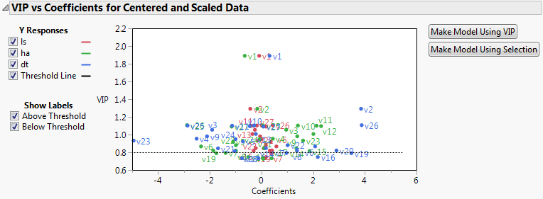
The VIP vs Coefficients plot helps identify variables that are influential relative to the fit for the various responses. For example, v23, v2, and v26 have both VIP values that exceed 0.8 and relatively large coefficients.
Launch the Partial Least Squares Platform
There are two ways to launch the Partial Least Squares platform:
• Select Analyze > Multivariate Methods > Partial Least Squares.
•  Select Analyze > Fit Model and select Partial Least Squares from the Personality menu. This approach enables you to do the following:
‒ Enter categorical variables as Ys or Xs. Conduct PLS-DA by entering categorical Ys.
‒ Add interaction and polynomial terms to your model.
‒ Use the Standardize X option to construct higher-order terms using centered and scaled columns.
‒ Save your model specification script.
Some features on the Fit Model launch window are not applicable for the Partial Least Squares personality:
• Weight, Nest, Attributes, Transform, and No Intercept.
Tip: You can transform a variable by right-clicking it in the Select Columns box and selecting a Transform option.
• The following Macros: Mixture Response Surface, Scheffé Cubic, and Radial.
Figure 6.6 JMP Pro Partial Least Squares Launch Window (Imputation Method EM Selected)

The Partial Least Squares launch window contains the following options:
Y, Response
Enter numeric response columns. If you enter multiple columns, they are modeled jointly.
X, Factor
Enter the predictor columns. The Partial Least Squares launch window only allows numeric predictors.
Freq
If your data are summarized, enter the column whose values contain counts for each row.
Enter an optional validation column. A validation column must contain only consecutive integer values. Note the following:
‒ If the validation column has two levels, the smaller value defines the training set and the larger value defines the validation set.
‒ If the validation column has three levels, the values define the training, validation, and test sets in order of increasing size.
‒ If the validation column has more than three levels, then KFold Cross Validation is used. For information about other validation options, see “Validation Method”.
Note: If you click the Validation button with no columns selected in the Select Columns list, you can add a validation column to your data table. For more information about the Make Validation Column utility, see Basic Analysis.
By
Enter a column that creates separate reports for each level of the variable.
Centering
Centers all Y variables and model effects by subtracting the mean from each column. See “Centering and Scaling”.
Scaling
Scales all Y variables and model effects by dividing each column by its standard deviation. See “Centering and Scaling”.
(Fit Model launch window only) Select this option to center and scale all columns that are used in the construction of model effects. If this option is not selected, higher-order effects are constructed using the original data table columns. Then each higher-order effect is centered or scaled, based on the selected Centering and Scaling options. Note that Standardize X does not center or scale Y variables. See “Standardize X”.
Replaces missing data values in Ys or Xs with nonmissing values. Select the appropriate method from the Imputation Method list.
If Impute Missing Data is not selected, rows that are missing observations on any X variable are excluded from the analysis and no predictions are computed for these rows. Rows with no missing observations on X variables but with missing observations on Y variables are also excluded from the analysis, but predictions are computed.
(Appears only when Impute Missing Data is selected) Select from the following imputation methods:
‒ Mean: For each model effect or response column, replaces the missing value with the mean of the nonmissing values.
‒ EM: Uses an iterative Expectation-Maximization (EM) approach to impute missing values. On the first iteration, the specified model is fit to the data with missing values for an effect or response replaced by their means. Predicted values from the model for Y and the model for X are used to impute the missing values. For subsequent iterations, the missing values are replaced by their predicted values, given the conditional distribution using the current estimates.
For the purpose of imputation, polynomial terms are treated as separate predictors. When a polynomial term is specified, that term is calculated from the original data, or, if Standardize X is checked, from the standardized column values. If a row has a missing value for a column involved in the definition of the polynomial term, then that entry is missing for the polynomial term. Imputation is conducted using polynomial terms defined in this way.
For more details about the EM approach, see Nelson, Taylor, and MacGregor (1996).
(Appears only when EM is selected as the Imputation Method) Enables you to set the maximum number of iterations used by the algorithm. The algorithm terminates if the maximum difference between the current and previous estimates of missing values is bounded by 10^-8.
After completing the launch window and clicking OK, the Model Launch control panel appears. See “Model Launch Control Panel”.
Centering and Scaling
The Centering and Scaling options are selected by default. This means that predictors and responses are centered and scaled to have mean 0 and standard deviation 1. Centering the predictors and the responses places them on an equal footing relative to their variation. Without centering, both the variable’s mean and its variation around that mean are involved in constructing successive factors. To illustrate, suppose that Time and Temp are two of the predictors. Scaling them indicates that a change of one standard deviation in Time is approximately equivalent to a change of one standard deviation in Temp.
Standardize X
Suppose that you have two columns, X1 and X2, and you enter the interaction term X1*X2 as a model effect in the Fit Model window. When the Standardize X option is selected, both X1 and X2 are centered and scaled before forming the interaction term. The interaction term that is formed is calculated as follows:

All model effects are then centered or scaled, in accordance with your selections of the Centering and Scaling options, prior to inclusion in the model.
If the Standardize X option is not selected, and Centering and Scaling are both selected, then the term that is entered into the model is calculated as follows:
Model Launch Control Panel
After you click OK in the platform launch window (or Run in the Fit Model window), the Model Launch control panel appears.
Figure 6.7 Partial Least Squares Model Launch Control Panel

Note: The Validation Method portion of the Model Launch control panel appears differently in JMP Pro.
The Model Launch control panel contains the following selections:
Method Specification
Select the type of model fitting algorithm. There are two algorithm choices: NIPALS and SIMPLS. The two methods produce the same coefficient estimates when there is only one response variable. See “Statistical Details” for details about differences between the two algorithms.
Validation Method
Select the validation method. Validation is used to determine the optimum number of factors to extract. For JMP Pro, if a validation column is specified on the platform launch window, these options do not appear.
Randomly selects the specified proportion of the data for a validation set, and uses the other portion of the data to fit the model.
Partitions the data into K subsets, or folds. In turn, each fold is used to validate the model that is fit to the rest of the data, fitting a total of K models. This method is best for small data sets because it makes efficient use of limited amounts of data.
Leave-One-Out
Performs leave-one-out cross validation.
None
Does not use validation to choose the number of factors to extract. The number of factors is specified in the Factor Search Range.
Factor Search Range
Specify how many latent factors to extract if not using validation. If validation is being used, this is the maximum number of factors the platform attempts to fit before choosing the optimum number of factors.
Factor Specification
Appears once you click Go to fit an initial model. Specify a number of factors to be used in fitting a new model.
Partial Least Squares Report
The first time you click Go in the Model Launch control panel (Figure 6.7), the Validation Method panel is removed from the Model Launch window. If you specified a Validation column or if you selected Holdback in the Validation Method panel, all model fits in the report are based on the training data. Otherwise, all model fits are based on the entire data set.
If you used validation, three reports appear:
• Model Comparison Summary
• <Cross Validation Method> and Method = <Method Specification>
• NIPALS (or SIMPLS) Fit with <N> Factors
If you selected None as the CV method, two reports appear:
• Model Comparison Summary
• NIPALS (or SIMPLS) Fit with <N> Factors
To fit additional models, specify the desired numbers of factors in the Model Launch panel.
Model Comparison Summary
The Model Comparison Summary shows summary results for each fitted model.
Figure 6.8 Model Comparison Summary

In Figure 6.8, models for 7 and then 6 factors have been fit. The report includes the following summary information:
Method
Shows the analysis method that you specified in the Model Launch control panel.
Number of rows
Shows the number of observations used in the training set.
Number of factors
Shows the number of extracted factors.
Percent Variation Explained for Cumulative X
Shows the percent of variation in X that is explained by the model.
Percent Variation Explained for Cumulative Y
Shows the percent of variation in Y that is explained by the model.
Number of VIP>0.8
Shows the number of model effects with VIP (variable importance for projection) values greater than 0.8. The VIP score is a measure of a variable’s importance relative to modeling both X and Y (Wold, 1995 and Eriksson et al., 2006).
<Cross Validation Method> and Method = <Method Specification>
This report appears only when a form of cross validation is selected as a Validation Method in the Model Launch control panel. It shows summary statistics for models fit, using from 0 to the maximum number of extracted factors, as specified in the Model Launch control panel. The report also provides a plot of Root Mean PRESS values. See “Root Mean PRESS Plot”. An optimum number of factors is identified using the minimum Root Mean PRESS statistic.
Figure 6.9 Cross Validation Report
The following statistics are shown in the report. If any form of validation or cross validation is used, the reported results are summaries of the training set statistics.
Number of Factors
Number of factors used in fitting the model.
Root Mean PRESS
The square root of the average of the PRESS values across all responses. For details, see “Root Mean PRESS”.
van der Voet T2
Test statistic for the van der Voet test, which tests whether models with different numbers of extracted factors differ significantly from the optimum model. The null hypothesis for each van der Voet T2 test states that the model based on the corresponding number of factors does not differ from the optimum model. The alternative hypothesis is that the model does differ from the optimum model. For more details, see “van der Voet T2”.
Prob > van der Voet T2
Q2
Dimensionless measure of predictive ability defined by subtracting the ratio of the PRESS value divided by the total sum of squares for Y from one:
Cumulative Q2
Indicator of the predictive ability of models with the given number of factors or fewer. For a given number of factors, f, Cumulative Q2 is defined as follows:

Here PRESSi and SSYi correspond to their values for i factors.
R2X
Percent of X variation explained by the specified factor. A component with a large R2X explains a large amount of the variation in the X variables. See “Calculation of R2X and R2Y When Validation Is Used”.
Cumulative R2X
Percent of X variation explained by the model with the given number of factors. This is the sum of the R2X values for i = 1 to the given number of factors.
R2Y
Percent of Y variation explained by the specified factor. A component with a large R2Y explains a large amount of the variation in the Y variables. See “Calculation of R2X and R2Y When Validation Is Used”.
Cumulative R2Y
Percent of Y variation explained by the model with the given number of factors. This is the Sum of the R2Y values for i = 1 to the given number of factors.
Interpretation of Q2 and Cumulative R2Y
The statistics Q2 and Cumulative R2Y both measure the predictive ability of the model, but in different ways.
• Cumulative R2Y increases as the number of factors increases. This is because, as factors are added to the model, more variation is explained.
• Q2 tends to increase and then decrease, or at least discontinue increasing, as the number of factors increases. This is because, as more factors are added, the model becomes tuned to the training set and does not generalize well to new data, causing the PRESS statistic to decrease.
Analysis of Q2 and Cumulative R2Y provides an alternative to using the van der Voet test for determining how many factors to include in your model. Select a number of factors for which Q2 is large and has not started decreasing. You also want Cumulative R2Y to be large.
Figure 6.10 shows plots of Cumulative R2Y and Q2 against the number of factors for the Penta.jmp data table, using Leave-One-Out as the validation method. Cumulative R2Y increases and levels off for about four factors. The statistic Q2 is largest for two factors and then begins to level off. The plot suggests that a model with two factors will explain a large portion of the variation in Y without overfitting the data.
Figure 6.10 Cumulative R2Y and Q2 for Penta.jmp

Root Mean PRESS Plot
This bar chart shows the number of factors along the horizontal axis and the Root Mean PRESS values on the vertical axis. It is equivalent to the horizontal bar chart that appears to the right of the Root Mean PRESS column in the Cross Validation report. See Figure 6.9.
Root Mean PRESS
For a specified number of factors, a, Root Mean PRESS is calculated as follows:
1. Fit a model with a factors to each training set.
2. Apply the resulting prediction formula to the observations in the validation set.
3. For each Y:
‒ For each validation set, compute the squared difference between each observed validation set value and its predicted value (the squared prediction error).
‒ For each validation set, average these squared differences and divide the result by a variance estimate for the response calculated as follows. For the KFold and Leave-One-Out validation methods, divide by the variance of the entire response column. For Holdback validation, divide by the variance of the response values in the training set.
‒ Sum these means and, in the case of more than one validation set, divide their sum by the number of validation sets minus one. This is the PRESS statistic for the given Y.
4. Root Mean PRESS for a factors is the square root of the average of the PRESS values across all responses.
5. The PRESS statistic for multiple Ys is obtained by averaging the PRESS statistic, obtained in step 3, across all responses.
Calculation of Q2
The statistic Q2 is defined as  . The PRESS statistic is the predicted error sum of squares averaged across all responses for the model developed based on the training data, but evaluated on the validation set. The value of SSY is the sum of squares for Y averaged across all responses and based on the observations in the validation set.
The statistic Q2 in the Cross Validation report is computed in the following ways, depending on the selected Validation Method:
Leave-One-Out
Q2 is the average of the values  computed for the validation sets based on the models constructed by leaving out one observation at a time.
KFold
Q2 is the average of the values  computed for the validation sets based on the K models constructed by leaving out each of the K folds.
Holdback or Validation Set
Q2 is the value of  computed for the validation set based on the model constructed using the single set of training data.
Calculation of R2X and R2Y When Validation Is Used
The statistics R2X and R2Y in the Cross Validation report are computed in the following ways, depending on the selected Validation Method:
Note: For all of these computations, R2Y is calculated analogously.
Leave-One-Out
R2X is the average of the Percent Variation Explained for X Effects for the models constructed by leaving out one observation at a time.
KFold
R2X is the average of the Percent Variation Explained for X Effects for the K models constructed by leaving out each fold.
Holdback or Validation Set
R2X is the Percent Variation Explained for X Effects for the model constructed using the training data.
Model Fit Report
The Model Fit Report shows detailed results for each fitted model. The fit uses either the optimum number of factors based on cross validation, or the specified number of factors if no cross validation methods are specified. The report title indicates whether NIPALS or SIMPLS was used and gives the number of extracted factors.
Figure 6.11 Model Fit Report

The Model Fit report includes the following summary information:
X-Y Scores Plots
Scatterplots of the X and Y scores for each extracted factor.
Percent Variation Explained
Shows the percent variation and cumulative percent variation explained for both X and Y. Results are given for each extracted factor.
Model Coefficients for Centered and Scaled Data
For each Y, shows the coefficients of the Xs for the model based on the centered and scaled data.
Partial Least Squares Options
The Partial Least Squares red triangle menu contains the following options:
Sets the seed for the randomization process used for KFold and Holdback validation. This is useful if you want to reproduce an analysis. Set the seed to a positive value, save the script, and the seed is automatically saved in the script. Running the script always produces the same cross validation analysis. This option does not appear when Validation Method is set to None, or when a validation column is used.
See the JMP Reports chapter in the Using JMP book for more information about the following options:
Redo
Contains options that enable you to repeat or relaunch the analysis. In platforms that support the feature, the Automatic Recalc option immediately reflects the changes that you make to the data table in the corresponding report window.
Save Script
Contains options that enable you to save a script that reproduces the report to several destinations.
Save By-Group Script
Contains options that enable you to save a script that reproduces the platform report for all levels of a By variable to several destinations. Available only when a By variable is specified in the launch window.
Model Fit Options
The Model Fit red triangle menu contains the following options:
Percent Variation Plots
Adds two plots entitled Percent Variation Explained for X Effects and Percent Variation Explained for Y Effects. These show stacked bar charts representing the percent variation explained by each extracted factor for the Xs and Ys.
Variable Importance Plot
Plots the VIP values for each X variable. VIP scores appear in the Variable Importance Table. See “Variable Importance Plot”.
VIP vs Coefficients Plots
Plots the VIP statistics against the model coefficients. You can show only those points corresponding to your selected Ys. Additional labeling options are provided. There are plots for both the centered and scaled data and the original data. See “VIP vs Coefficients Plots”.
Set VIP Threshold
Sets the threshold level for the Variable Importance Plot, Variance Importance Table, and the VIP vs Coefficients Plots.
Coefficient Plots
Plots the model coefficients for each response across the X variables. You can show only those points corresponding to your selected Ys. There are plots for both the centered and scaled data and the original data.
Loading Plots
Plots X and Y loadings for each extracted factor. There are separate plots for the Xs and Ys.
Loading Scatterplot Matrices
Shows scatterplot matrices of the X loadings and the Y loadings.
Correlation Loading Plot
Shows either a single scatterplot or a scatterplot matrix of the X and Y loadings overlaid on the same plot. When you select the option, you specify how many factors you want to plot.
‒ If you specify two factors, a single correlation loading scatterplot appears. Select the two factors that define the axes beneath the plot. Click the right arrow button to successively display each combination of factors on the plot.
‒ If you specify more than two factors, a scatterplot matrix appears with a cell for pair of factors up to the number that you selected.
In both cases, use check boxes to control labeling.
X-Y Score Plots
Includes the following options:
Fit Line Shows or hides a fitted line through the points on the X-Y Scores Plots.
Show Confidence Band Shows or hides 95% confidence bands for the fitted lines on the X-Y Scores Plots. These should be used only for outlier detection.
Score Scatterplot Matrices
Shows a scatterplot matrix of the X scores and a scatterplot matrix of the Y scores. Each X score scatterplot displays a 95% confidence ellipse, which can be used for outlier detection. For statistical details about the confidence ellipses, see “Confidence Ellipses for X Score Scatterplot Matrix”.
Distance Plots
Shows plots of the following:
‒ the distance from each observation to the X model
‒ the distance from each observation to the Y model
‒ a scatterplot of distances to both the X and Y models
In a good model, both X and Y distances are small, so the points are close to the origin (0,0). Use the plots to look for outliers relative to either X or Y. If a group of points clusters together, then they might have a common feature and could be analyzed separately. When a validation set or a validation and test set are in use, separate reports are provided for these sets and for the training set.
T Square Plot
Shows a plot of T2 statistics for each observation, along with a control limit. An observation’s T2 statistic is calculated based on that observation’s scores on the extracted factors. For details about the computation of T2 and the control limit, see “T2 Plot”.
Diagnostics Plots
Shows diagnostic plots for assessing the model fit. Four plot types are available: Actual by Predicted Plot, Residual by Predicted Plot, Residual by Row Plot, and a Residual Normal Quantile Plot. Plots are provided for each response. When a validation set or a validation and test set are in use, separate reports are provided for these sets and for the training set.
Profiler
shows a profiler for each Y variable.
Spectral Profiler
Shows a single profiler where all of the response variables appear in the first cell of the plot. This profiler is useful for visualizing the effect of changes in the X variables on the Y variables simultaneously.
Save Columns
Includes options for saving various formulas and results. See “Save Columns”.
Remove Fit
Removes the model report from the main platform report.
Make Model Using VIP
Opens and populates a launch window with the appropriate responses entered as Ys and the variables whose VIPs exceed the specified threshold entered as Xs. Performs the same function as the button in the VIP vs Coefficients for Centered and Scaled Data report. See “VIP vs Coefficients Plots”.
Variable Importance Plot
The Variable Importance Plot graphs the VIP values for each X variable. The Variable Importance Table shows the VIP scores. A VIP score is a measure of a variable’s importance in modeling both X and Y. If a variable has a small coefficient and a small VIP, then it is a candidate for deletion from the model (Wold,1995). A value of 0.8 is generally considered to be a small VIP (Eriksson et al, 2006) and a red dashed line is drawn on the plot at 0.8.
Figure 6.12 Variable Importance Plot

VIP vs Coefficients Plots
Two options to the right of the plot facilitate variable reduction and model building:
• Make Model Using VIP opens and populates a launch window with the appropriate responses entered as Ys and the variables whose VIPs exceed the specified threshold entered as Xs.
• Make Model Using Selection enables you to select Xs directly in the plot and then enters the Ys and only the selected Xs into a launch window.
To use another platform based on your current column selection, open the desired platform. Notice in the launch window that the selections are retained. Click on the role button and the selected columns are populated.
Figure 6.13 VIP vs Coefficients Plot for Centered and Scaled Data
Save Columns
Save Prediction Formula
For each Y variable, saves a column to the data table called Pred Formula <response> that contains its the prediction formula.
Save Prediction as X Score Formula
For each Y variable, saves a column to the data table called Pred Formula <response> that contains the prediction formula in terms of the X scores.
Save Standard Errors of Prediction Formula
For each Y variable, saves a column to the data table called PredSE <response> that contains the standard error of the predicted mean. For details, see “Standard Error of Prediction and Confidence Limits”.
Save Mean Confidence Limit Formula
For each Y variable, saves two columns to the data table called Lower 95% Mean <response> and Upper 95% Mean <response>. These columns contain 95% confidence limits for the response mean. For details, see “Standard Error of Prediction and Confidence Limits”.
Save Indiv Confidence Limit Formula
For each Y variable, saves two columns to the data table called Lower 95% Indiv <response> and Upper 95% Indiv <response>. These columns contain 95% prediction limits for individual values. For details, see “Standard Error of Prediction and Confidence Limits”.
Save Score Formula
Saves two sets of columns to the data table:
‒ Columns called X Score <N> Formula containing the formulas for each X Score.
‒ Columns called Y Score <N> Formula containing the formulas for each Y Score
Save Y Predicted Values
Saves the predicted values for the Y variables to columns in the data table.
Save Y Residuals
Saves the residual values for the Y variables to columns in the data table.
Save X Predicted Values
Saves the predicted values for the X variables to columns in the data table.
Save X Residuals
Saves the residual values for the X variables to columns in the data table.
Save Percent Variation Explained For X Effects
Saves the percent variation explained for each X variable across all extracted factors to a new data table.
Save Percent Variation Explained For Y Responses
Saves the percent variation explained for each Y variable across all extracted factors to a new data table.
Save Scores
Saves the X and Y scores for each extracted factor to the data table.
Save Loadings
Saves the X and Y loadings to new data tables.
Save Standardized Scores
Saves the X and Y standardized scores used in constructing the Correlation Loading Plot to the data table. For the formulas, see “Standardized Scores and Loadings”.
Save Standardized Loadings
Saves the X and Y standardized loadings used in constructing the Correlation Loading Plot to new data tables. For the formulas, see “Standardized Scores and Loadings”.
Save T Square
Saves the T2 values to the data table. These are the values used in the T Square Plot.
Save Distance
Saves the Distance to X Model (DModX) and Distance to Y Model (DModY) values to the data table. These are the values used in the Distance Plots.
Save X Weights
Saves the weights for each X variable across all extracted factors to a new data table.
Saves a new column to the data table describing how each observation was used in validation. For Holdback validation, the column identifies if a row was used for training or validation. For KFold validation, the column identifies the number of the subgroup to which the row was assigned.
If Impute Missing Data is selected, opens a new data table that contains the data table columns specified as X and Y, with missing values replaced by their imputed values. Columns for polynomial terms are not shown. If a Validation column is specified, the validation column is also included.
Creates prediction formulas and saves them as formula column scripts in the Formula Depot platform. If a Formula Depot report is not open, this option creates a Formula Depot report. See the Formula Depot chapter in the Predictive and Specialized Modeling book.
Creates X and Y score formulas and saves them as formula column scripts in the Formula Depot platform. If a Formula Depot report is not open, this option creates a Formula Depot report. See the Formula Depot chapter in the Predictive and Specialized Modeling book.
Statistical Details
This section provides details about some of the methods used in the Partial Least Squares platform. For additional details, see Hoskuldsson (1988), Garthwaite (1994), or Cox and Gaudard (2013).
Partial Least Squares
Partial least squares fits linear models based on linear combinations, called factors, of the explanatory variables (Xs). These factors are obtained in a way that attempts to maximize the covariance between the Xs and the response or responses (Ys). In this way, PLS exploits the correlations between the Xs and the Ys to reveal underlying latent structures. The factors address the combined goals of explaining response variation and predictor variation. Partial least squares is particularly useful when you have more X variables than observations or when the X variables are highly correlated.
NIPALS
The NIPALS method works by extracting one factor at a time. Let X = X0 be the centered and scaled matrix of predictors and Y = Y0 the centered and scaled matrix of response values. The PLS method starts with a linear combination t = X0w of the predictors, where t is called a score vector and w is its associated weight vector. The PLS method predicts both X0 and Y0 by regression on t:
The vectors p and c are called the X- and Y-loadings, respectively.
The specific linear combination t = X0w is the one that has maximum covariance t´u with some response linear combination u = Y0q. Another characterization is that the X- and Y-weights, w and q, are proportional to the first left and right singular vectors of the covariance matrix X0´Y0. Or, equivalently, the first eigenvectors of X0´Y0Y0´X0 and Y0´X0X0´Y0 respectively.
This accounts for how the first PLS factor is extracted. The second factor is extracted in the same way by replacing X0 and Y0 with the X- and Y-residuals from the first factor:
X1 = X0 –
Y1 = Y0 –
These residuals are also called the deflated X and Y blocks. The process of extracting a score vector and deflating the data matrices is repeated for as many extracted factors as desired.
SIMPLS
The SIMPLS algorithm was developed to optimize a statistical criterion: it finds score vectors that maximize the covariance between linear combinations of Xs and Ys, subject to the requirement that the X-scores are orthogonal. Unlike NIPALS, where the matrices X0 and Y0 are deflated, SIMPLS deflates the cross-product matrix, X0´Y0.
In the case of a single Y variable, these two algorithms are equivalent. However, for multivariate Y, the models differ. SIMPLS was suggested by De Jong (1993).
van der Voet T2
The van der Voet T2 test helps determine whether a model with a specified number of extracted factors differs significantly from a proposed optimum model. The test is a randomization test based on the null hypothesis that the squared residuals for both models have the same distribution. Intuitively, one can think of the null hypothesis as stating that both models have the same predictive ability.
To obtain the van der Voet T2 statistic given in the Cross Validation report, the calculation below is performed on each validation set. In the case of a single validation set, the result is the reported value. In the case of Leave-One-Out and KFold validation, the results for each validation set are averaged.
Denote by  the jth predicted residual for response k for the model with i extracted factors. Denote by
  is the corresponding quantity for the model based on the proposed optimum number of factors, opt. The test statistic is based on the following differences:
Suppose that there are K responses. Consider the following notation:


The van der Voet statistic for i extracted factors is defined as follows:
The significance level is obtained by comparing Ci with the distribution of values that results from randomly exchanging  and
and  . A Monte Carlo sample of such values is simulated and the significance level is approximated as the proportion of simulated critical values that are greater than or equal to Ci.
T2 Plot
The T2 value for the ith observation is computed as follows:

where tij = X score for the ith row and jth extracted factor, p = number of extracted factors, and n = number of observations used to train the model. If validation is not used, n = total number of observations.
The control limit for the T2 Plot is computed as follows:
((n-1)2/n)*BetaQuantile(0.95, p/2, (n-p-1)/2)
where p = number of extracted factors, and n = number of observations used to train the model. If validation is not used, n = total number of observations. See Tracy, Young, and Mason, 1992.
Confidence Ellipses for X Score Scatterplot Matrix
The Score Scatterplot Matrices option adds 95% confidence ellipses to the X Score scatterplots. The X scores are uncorrelated because both the NIPALS and SIMPLE algorithms produce orthogonal score vectors. The ellipses assume that each pair of X scores follows a bivariate normal distribution with zero correlation.
Consider a scatterplot for score i on the vertical axis and score j on the horizontal axis. The coordinates of the top, bottom, left, and right extremes of the ellipse are as follows:
• the top and bottom extremes are +/-sqrt(var(score i)*z)
• the left and right extremes are +/-sqrt(var(score j)*z)
where z = ((n-1)*(n-1)/n)*BetaQuantile(0.95, 1, (n-3)/2). For background on the z value, see Tracy, Young, and Mason, 1992.
Standard Error of Prediction and Confidence Limits
Let X denote the matrix of predictors and Y the matrix of response values, which might be centered and scaled based on your selections in the launch window. Assume that the components of Y are independent and normally distributed with a common variance σ2.
Hoskuldsson (1988) observes that the PLS model for Y in terms of scores is formally similar to a multiple linear regression model. He uses this similarity to derive an approximate formula for the variance of a predicted value. See also Umetrics (1995). However, Denham (1997) points out that any value predicted by PLS is a non-linear function of the Ys. He suggests bootstrap and cross validation techniques for obtaining prediction intervals. The PLS platform uses the normality-based approach described in Umetrics (1995).
Denote the matrix whose columns are the scores by T and consider a new observation on X, x0. The predictive model for Y is obtained by regressing Y on T. Denote the score vector associated with x0 by t0.
Let a denote the number of factors. Define s2 to be the sum of squares of residuals divided by df = n - a -1 if the data are centered and df = n - a if the data are not centered. The value of s2 is an estimate of σ2.
Standard Error of Prediction Formula
The standard error of the predicted mean at x0 is estimated by the following:

Mean Confidence Limit Formula
Let t0.975, df denote the 0.975 quantile of a t distribution with degrees of freedom df = n - a -1 if the data are centered and df = n - a if the data are not centered.
The 95% confidence interval for the mean is computed as follows:
Indiv Confidence Limit Formula
The standard error of a predicted individual response at x0 is estimated by the following:

Let t0.975, df denote the 0.975 quantile of a t distribution with degrees of freedom df = n - a -1 if the data are centered and df = n - a if the data are not centered.
The 95% prediction interval for an individual response is computed as follows:
Standardized Scores and Loadings
Consider the following notation:
• ntr is the number of observations in the training set
• m is the number of effects in X
• k is the number of responses in Y
• VarXi is the percent variation in X explained by the ith factor
• VarYi is the percent variation in Y explained by the ith factor
• XScorei is the vector of X scores for the ith factor
• YScorei is the vector of Y scores for the ith factor
• XLoadi is the vector of X loadings for the ith factor
• YLoadi is the vector of Y loadings for the ith factor
Standardized Scores
The vector of ith Standardized X Scores is defined as follows:

The vector of ith Standardized Y Scores is defined as follows:

Standardized Loadings
The vector of ith Standardized X Loadings is defined as follows:
The vector of ith Standardized Y Loadings is defined as follows:
PLS Discriminant Analysis (PLS-DA)
When a categorical variable is entered as Y in the launch window, it is coded using indicator coding. If there are k levels, each level is represented by an indicator variable with the value 1 for rows in that level and 0 otherwise. The resulting k indicator variables are treated as continuous and the PLS analysis proceeds as it would with continuous Ys.
..................Content has been hidden....................
You can't read the all page of ebook, please click here login for view all page.