
Chapter 4
Advanced Disk Management
THE FOLLOWING LINUX PROFESSIONAL INSTITUTE OBJECTIVES ARE COVERED IN THIS CHAPTER:
- 204.1 Configuring RAID (weight: 2)
- 204.2 Adjusting Storage Device Access (weight: 1)
- 204.3 Logical Volume Manager (weight: 3)
- 206.2 Backup operations (weight: 3)
 Chapter 3, “Basic Filesystem Management,” describes how to create and manage filesystems. The topic of managing filesystems is tied closely to the topic of managing the data structures that contain them. Most commonly, these data structures are partitions—contiguous collections of sectors on a hard disk. Partition management is covered in the LPIC-1 exams. LPIC-2, and therefore this chapter, emphasizes more advanced filesystem container management: Redundant Array of Independent Disks (RAID), which enables merging multiple disks together to improve performance or security; and Logical Volume Manager (LVM), which enables combining partitions or disks into a storage area that can be managed more flexibly than conventional partitions. Although the LPIC-2 exam emphasizes these topics, the fact that they rely on simple partitions means that this chapter begins with information on conventional partitioning.
This chapter also covers additional disk-related topics. The first of these is adjusting hardware parameters for optimal performance. Typically, Linux performs reasonably well with no modifications; however, it's sometimes possible to improve performance by using various utilities. Another important topic is that of backing up your data. Without a backup, a failure of disk hardware or corruption of filesystem data structures can make for a very bad day, so preparing for such a problem is extremely important.
Partitioning Disks
Hard disks are typically broken into segments, known as partitions, that can be used for various purposes. In Linux, most partitions (or, to be more precise, the filesystems they contain) are mounted at specific directories. Swap partitions are an exception to this rule; they are accessed as an adjunct to system memory. Although Chapter 3 describes filesystem and swap space management, it doesn't describe partition management. The next few pages describe this topic, including both the important principles and partition types and the basic operation of the tools used to create partitions.
Understanding Partitions
Partitions are described in a data structure that is known generically as a partition table. The partition table is stored in one or more sectors of a hard disk, in locations that are defined by the partition table type. Over the years, several different partition table types have been developed. In 2010, three partition table types are most important:
Master Boot Record (MBR) This partition table type is the most common one on disks under 2 TiB in size. It was used by Microsoft's Disk Operating System (DOS) and has been adopted by most OSs that run on the same hardware as DOS and its successor, Windows. Unfortunately, MBR suffers from many limitations, as described shortly, and so is being slowly abandoned. MBR is known by various other names, including MS-DOS partitions and BIOS partitions.
Apple Partition Map (APM) Apple used this partition table type on its 680x0- and PowerPC-based Macintoshes, and it's been adopted by a few other computer types. Because Mac OS has never dominated the marketplace, APM is uncommon except on older Mac hardware; however, you may occasionally run into a removable disk that uses APM.
GUID Partition Table (GPT) This partition table type is described in the Extensible Firmware Interface (EFI) definition, but it can be used on non-EFI systems. Apple switched to GPT for its Macintosh computers when it adopted Intel CPUs. GPT overcomes many of the problems of the older MBR and APM partition tables, particularly their disk size limits, and so GPT seems likely to become increasingly important as disk sizes rise.
Most Linux computers use MBR partitions; however, if you're running Linux on a PowerPC-based Mac, it probably uses APM. Newer Macs, and some non-Mac systems, use GPT.
As just noted, MBR has a number of limitations. The most important of these is that it uses 32-bit pointers to refer to disk sectors. Given a sector size of 512 bytes, this works out to a limit on partition size of precisely 2 TiB (232 × 512 bytes = 2.2 × 1012 bytes, or 2 TiB). APM shares the same limit. GPT, by contrast, uses 64-bit sector pointers, so it can handle disks of up to 9.4 × 1021 bytes—8 ZiB (zebibytes).
![]() Disk manufacturers are beginning to transition away from 512-byte sectors to 4096-byte sectors. This change may extend the useful life of MBR, since its limit is raised to 16 TiB with 4096-byte sectors.
Disk manufacturers are beginning to transition away from 512-byte sectors to 4096-byte sectors. This change may extend the useful life of MBR, since its limit is raised to 16 TiB with 4096-byte sectors.
MBR has some other quirks that deserve mention. The first of these is that the original MBR specification provided for just four partitions. When this limit became troublesome, a workaround was devised: One of the original four partitions (now known as primary partitions) was allocated as a placeholder (an extended partition) for an arbitrary number of additional partitions (logical partitions). Although this is an effective workaround, it can be limiting. All logical partitions must reside within a single extended partition, which means that primary partitions cannot exist between logical partitions. As a disk is used, it's common to want to delete, add, move, and resize partitions, and these operations can become awkward when working around the primary/extended/logical partition requirements. Furthermore, some OSs, such as Microsoft Windows, must boot from a primary partition. (Linux is not so limited.) In Linux, primary partitions are numbered from 1 to 4, while logical partitions are numbered 5 and up.
GPT uses a different set of data structures than does MBR, so GPT's limits and quirks are different. Under GPT, there is no distinction between primary, extended, and logical partitions. Instead, GPT supports a fixed number of partitions (128 by default), all of which are defined in the main partition table. GPT and MBR support slightly different meta-data—for instance, GPT supports a partition name, which MBR doesn't support.
No matter what partitioning system you use, you should be aware of one critical limitation of partitions: They are composed of contiguous sets of sectors. Thus, if you want to change the way partitions are laid out, you may need to move all the data on one or more partitions. This is one of the limitations that LVM is designed to overcome, as described later in “Configuring LVM.”
Creating Partitions
Several Linux tools are available to partition MBR and GPT disks in Linux:
The libparted Tools The GNU Project's libparted (http://www.gnu.org/software/parted/), which comes with the parted text-mode program, is a popular tool that can handle MBR, GPT, APM, and several other partition table formats. GUI tools, such as GNOME Partition Editor (aka GParted; http://gparted.sourceforge.net), have been built upon libparted. The greatest strength of these tools is the ability to move and resize both partitions and the filesystems they contain. They can also create filesystems at the same time you create partitions.
The fdisk Family The Linux fdisk program is named after the DOS FDISK program. Although the two are very different in operation, they do the same basic job: They create and manipulate MBR partition tables. In Linux, fdisk is the basic program, with a simple text-mode interactive user interface. The sfdisk program can do similar jobs, but it's designed to be used in a non-interactive way via command-line options. It's therefore useful in scripts. The cfdisk program uses a more sophisticated text-mode interface similar to that of a text editor. These programs ship with the standard util-linux or util-linux-ng packages.
GPT fdisk This package, consisting of the gdisk and sgdisk programs, is designed as a workalike to fdisk but for GPT disks. The gdisk program is modeled on fdisk. Although sgdisk is designed for shell-based interaction, it bears little resemblance to sfdisk in its operational details. You can learn more at http://www.rodsbooks.com/gdisk/.
Partitions can be created, deleted, and otherwise manipulated using any of these programs (or other programs for other partition table types). In most cases, you launch the program by typing its name followed by a disk device filename, such as /dev/sda. You'll then see a command prompt, such as the following for fdisk:
Command (m for help):
![]() If fdisk displays a message to the effect that GPT was detected on the disk, exit immediately by typing q! You should use GPT fdisk or a libparted-based tool on such disks. Attempting to use fdisk on a GPT disk is likely to cause serious problems.
If fdisk displays a message to the effect that GPT was detected on the disk, exit immediately by typing q! You should use GPT fdisk or a libparted-based tool on such disks. Attempting to use fdisk on a GPT disk is likely to cause serious problems.
Pass fdisk the -u option to have it use sectors rather than cylinders as the default units of measure. Passing -c affects where fdisk starts its first partition. As a general rule, both options are desirable on modern disks, so you should generally launch it as fdisk -uc /dev/sda (changing the device filename, if necessary).
Table 4.1 summarizes the most important fdisk commands that can be typed at this prompt. Some of these commands silently do something, but others require interaction. For instance, typing n results in a series of prompts for the new partition's type (primary, extended, or logical), start point, and size or end point. (If you must edit a GPT disk, gdisk supports all the commands shown in Table 4.1 except u, although some of the details of subsequent interactions differ slightly.)
TABLE 4.1 Common fdisk commands
| Command | Explanation |
| d | Deletes a partition. |
| l | Displays a list of partition type codes |
| n | Creates a new partition |
| o | Destroys the current partition table, enabling you to start fresh |
| p | Displays the current partition table |
| q | Exits without saving changes |
| t | Changes a partition's type code |
| u | Toggles units between sectors and cylinders |
| v | Performs checks on the validity of the disk's data structures |
| w | Saves changes and exits |
The l and t commands deserve elaboration: MBR supports a 1-byte type code for each partition. This code helps identify what types of data are supposed to be stored on the partition. For instance, in hexadecimal, 0x07 refers to a partition that holds High Performance Filesystem (HPFS) or New Technology Filesystem (NTFS) data, 0x82 refers to a Linux swap partition, and 0x83 refers to a Linux data partition. For the most part, Linux ignores partition type codes; however, Linux installers frequently rely on them, as do other OSs. Thus, you should be sure your partition type codes are set correctly. Linux fdisk creates 0x83 partitions by default, so you should change the code if you create anything but a Linux partition.
![]() If you just want to view the partition table, type fdisk -lu /dev/sda. This command displays the partition table, using units of sectors, and then exits. You can change the device filename for the device in which you're interested, of course.
If you just want to view the partition table, type fdisk -lu /dev/sda. This command displays the partition table, using units of sectors, and then exits. You can change the device filename for the device in which you're interested, of course.
GPT also supports partition type codes, but these codes are 16-byte GUID values rather than 1-byte MBR type codes. GPT fdisk translates the 16-byte GUIDs into 2-byte codes based on the MBR codes; for instance, the GPT code for a Linux swap partition becomes 0x8200. Unfortunately, Linux and Windows use the same GUID code for their partitions, so GPT fdisk translates both to 0x0700. Programs based on libparted don't give direct access to partition type codes, although they use them internally. Several GPT type codes are referred to as “flags” in libparted-based programs; for instance, the “boot flag” refers to a partition with the type code for an EFI System Partition on a GPT disk.
Configuring RAID
In a RAID configuration, multiple disks are combined together to improve performance, reliability, or both. The following pages describe RAID in general, Linux's RAID subsystem, preparing a disk for use with RAID, initializing the RAID structures, and using RAID disks.
Understanding RAID
The purpose of RAID depends on its specific level:
Linear Mode This isn't technically RAID, but it's handled by Linux's RAID subsystem. In linear mode, devices are combined together by appending one device's space to another's. Linear mode provides neither speed nor reliability benefits, but it can be a quick way to combine disk devices if you need to create a very large filesystem. The main advantage of linear mode is that you can combine partitions of unequal size without losing storage space; other forms of RAID require equal-sized underlying partitions and ignore some of the space if they're fed unequal-sized partitions.
RAID 0 (Striping) This form of RAID combines multiple disks to present the illusion of a single storage area as large as all the combined disks. The disks are combined in an interleaved manner so that a single large access to the RAID device (for instance, when reading or writing a large file) results in accesses to all the component devices. This configuration can improve overall disk performance; however, if any one disk fails, data on the remaining disks will become useless. Thus, reliability actually decreases when using RAID 0, compared to conventional partitioning.
![]() LVM provides a striping feature similar to RAID 0. Thus, if you want to use striping and LVM, you can skip the RAID configuration and use LVM alone. If you're interested only in striping, you can use either RAID 0 or LVM.
LVM provides a striping feature similar to RAID 0. Thus, if you want to use striping and LVM, you can skip the RAID configuration and use LVM alone. If you're interested only in striping, you can use either RAID 0 or LVM.
RAID 1 (Mirroring) This form of RAID creates an exact copy of one disk's contents on one or more other disks. If any one disk fails, the other disks can take over, thus improving reliability. The drawback is that disk writes take longer, since data must be written to two or more disks. Additional disks may be assigned as hot standby or hot spare disks, which can automatically take over from another disk if one fails. (Higher RAID levels also support hot standby disks.)
![]() Hot spare disks are normally inactive; they come into play only in the event another disk fails. As a result, when a failure occurs, the RAID subsystem must copy data onto the hot spare disk, which takes time.
Hot spare disks are normally inactive; they come into play only in the event another disk fails. As a result, when a failure occurs, the RAID subsystem must copy data onto the hot spare disk, which takes time.
RAID 4 Higher levels of RAID attempt to gain the benefits of both RAID 0 and RAID 1. In RAID 4, data are striped in a manner similar to RAID 0; but one drive is dedicated to holding checksum data. If any one disk fails, the checksum data can be used to regenerate the lost data. The checksum drive does not contribute to the overall amount of data stored; essentially, if you have n identically sized disks, they can store the same amount of data as n – 1 disks of the same size in a non-RAID or RAID 0 configuration. As a practical matter, you need at least three identically sized disks to implement a RAID 4 array.
RAID 5 This form of RAID works just like RAID 4, except that there's no dedicated checksum drive; instead, the checksum data are interleaved on all the disks in the array. RAID 5's size computations are the same as those for RAID 4; you need a minimum of three disks, and n disks hold n – 1 disks worth of data.
RAID 6 What if two drives fail simultaneously? In RAID 4 and RAID 5, the result is data loss. RAID 6, though, increases the amount of checksum data, therefore increasing resistance to disk failure. The cost, however, is that you need more disks: four at a minimum. With RAID 6, n disks hold n – 2 disks worth of data.
RAID 10 A combination of RAID 1 with RAID 0, referred to as RAID 1 + 0 or RAID 10, provides benefits similar to those of RAID 4 or RAID 5. Linux provides explicit support for this combination to simplify configuration.
![]() Additional RAID levels exist; however, the Linux kernel explicitly supports only the preceding RAID levels. If you use a hardware RAID disk controller, as described shortly in the Real World Scenario “Software vs. Hardware RAID,” you might encounter other RAID levels.
Additional RAID levels exist; however, the Linux kernel explicitly supports only the preceding RAID levels. If you use a hardware RAID disk controller, as described shortly in the Real World Scenario “Software vs. Hardware RAID,” you might encounter other RAID levels.
Linux's implementation of RAID is usually applied to partitions rather than to whole disks. Partitions are combined by the kernel RAID drivers to create new devices, with names of the form /dev/md#, where # is a number from 0 up. This configuration enables you to combine devices using different RAID levels, to use RAID for only some partitions, or even to use RAID with disks of different sizes. For instance, suppose you have two 1.5 TiB disks and one 2 TiB disk. You could create a 2 TiB RAID 4 or RAID 5 array using 1 TiB partitions on each of the disks, a 1 TiB RAID 0 array using 0.5 TiB from one of the 1.5 TiB disk and the 2 TiB disk, and a 0.5 TiB RAID 1 array using 0.5 TiB from the second 1.5 TiB disk and the 2 TiB disk.
When using Linux's software RAID, you should realize that boot loaders are sometimes unable to read RAID arrays. GRUB Legacy, in particular, can't read data in a RAID array. (RAID 1 is a partial exception; because RAID 1 partitions are duplicates of each other, GRUB Legacy can treat them like normal partitions for read-only access.) GRUB 2 includes Linux RAID support, however. Because of this limitation, you may want to leave a small amount of disk space in a conventional partition or used as RAID 1, for use as a Linux /boot partition.
When you partition a disk for RAID, you should be sure to assign the proper partition type code. On an MBR disk, this is 0xFD. If you edit a GPT disk using GPT fdisk, the equivalent code is 0xFD00. If you use a libparted-based tool with either MBR or GPT disks, a RAID partition is identified as one with the RAID flag set.
RAID relies on Linux kernel features. Most distributions ship with kernels that have the necessary support. If you compile your own kernel, however, as described in Chapter 2, “Linux Kernel Configuration,” you should be sure to activate the RAID features you need. These can be found in the Device Drivers ![]() Multiple Devices Driver Support (RAID and LVM)
Multiple Devices Driver Support (RAID and LVM) ![]() RAID Support area. Enable the main RAID Support area along with support for the specific RAID level or levels you intend to use. It's best to compile this support directly into the kernel, since this can sometimes obviate the need to create an initial RAM disk.
RAID Support area. Enable the main RAID Support area along with support for the specific RAID level or levels you intend to use. It's best to compile this support directly into the kernel, since this can sometimes obviate the need to create an initial RAM disk.

Software vs. Hardware RAID
This chapter emphasizes Linux's software RAID subsystem; however, RAID can also be implemented by special disk controllers with hardware RAID support. When using such a controller, multiple hard disks appear to Linux to be single disks with a conventional disk device filename, such as /dev/sda.
Generally speaking, hardware RAID implementations are more efficient than software RAID implementations. This is particularly true of RAID 1; a hardware RAID controller is likely to enable true parallel access to both drives, with no extra overhead. Hardware RAID also computes the checksums required for higher RAID levels, removing this burden from the CPU.
Be aware that many motherboards claim to have built-in RAID support. Most of these, however, implement their own proprietary form of software RAID, which some people refer to as fake RAID. These implementations require special drivers, which may or may not be available for Linux. As a general rule, it's better to use Linux's own software RAID implementations. If you want the benefits of true hardware RAID, you will probably have to buy a new disk controller. Be sure that the Linux kernel supports any hardware RAID controller you buy.
If you have a true hardware RAID controller, you should consult its documentation to learn how to configure it. Once it's set up, it should present the illusion of one disk that's larger than any of your individual disks. There is then no need to apply Linux's software RAID features; you can partition and use the hardware RAID array as if it were a single conventional disk.
Disks in a hardware RAID array are accessed in blocks, typically between 16 KiB and 256 KiB in size. This block size is larger than the 512-byte sector size, and this fact can have performance implications. In particular, if partitions do not start on multiples of the RAID array allocation block, performance can be degraded by 10–30 percent. The latest versions of Linux partitioning software provide options to align partitions on 1 MiB boundaries, which is a safe default for such devices. Be sure you use such an option if you use a hardware RAID controller.
Preparing a Disk for Software RAID
The first step in software RAID configuration is partitioning the disk. As noted earlier, you should give the partitions the correct type code in fdisk or any other partitioning software you're using. Two methods of partitioning for RAID are possible:
- You can create a single RAID partition on each disk and then, when you've defined the full array, create partitions in it as if the RAID array were a hard disk.
- You can create multiple partitions on the underlying disk devices, assembling each into a separate RAID device that will be used to store a filesystem.
The first method can simplify the initial RAID configuration, but the second method is more flexible; using the second method enables you to use different RAID levels or even combine disks of unequal size into your RAID configuration.
![]() When you define RAID partitions, be sure that the partitions to be combined on multiple disks are as equal in size as possible. If the component partitions are of unequal size, only the amount of space in the smallest partition will be used in all the others. For instance, if you combine an 800 MiB partition on one disk with two 900 MiB partitions on two other disks, you'll be throwing away 100 MiB of space on each of the two disks with 900 MiB partitions. Sometimes a small amount of waste is acceptable if your disks have slightly different sizes. If the amount of wasted space is significant, though, you might want to use the otherwise wasted space as conventional (non-RAID) partitions.
When you define RAID partitions, be sure that the partitions to be combined on multiple disks are as equal in size as possible. If the component partitions are of unequal size, only the amount of space in the smallest partition will be used in all the others. For instance, if you combine an 800 MiB partition on one disk with two 900 MiB partitions on two other disks, you'll be throwing away 100 MiB of space on each of the two disks with 900 MiB partitions. Sometimes a small amount of waste is acceptable if your disks have slightly different sizes. If the amount of wasted space is significant, though, you might want to use the otherwise wasted space as conventional (non-RAID) partitions.
Normally, disks to be combined using RAID will be of the same size. If you're stuck with unequal-sized disks, you can leave some space on the larger disks outside of the RAID array or, with enough disks, find ways to combine segments from subsets of the disks. (Linear mode enables combining disks of unequal size.)
If you're using older Parallel Advanced Technology Attachment (PATA) disks, which enable two disks to be connected via a single cable, it's best to combine devices on different cables into a single RAID array. The reason is that PATA bandwidth is limited on a per-channel basis, so combining two devices on a single channel (that is, one cable) will produce a smaller performance benefit than combining devices on different channels. Newer Serial ATA (SATA) disks don't have this problem because SATA supports one device per channel. Small Computer Systems Interface (SCSI) devices multitask well even on a single channel.
Assembling a RAID Array
Once you've set up the partitions that are to be included in a RAID array, you may use the mdadm tool to define how the devices should be assembled. (This tool's name is short for multiple device administration.) This command's syntax is:
mdadm [mode] raid-device [options] component-devices
Table 4.2 summarizes the mode values you may use, while Table 4.3 summarizes the most important options. Most of your use of mdadm will employ the --create mode; other options are intended for troubleshooting, advanced use, or reconfiguring an already-created RAID array. (The --auto-detect mode is called by startup scripts when the system boots.) If no mode is specified, the command is in manage mode or misc mode; various miscellaneous tasks can be performed in these modes.
TABLE 4.2 Common mode values for mdadm
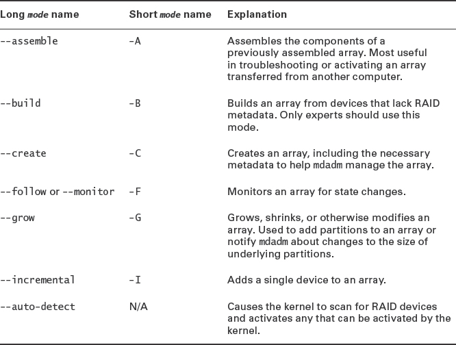
TABLE 4.3 Common options for mdadm
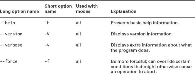

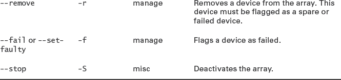
Table 4.3 is incomplete; mdadm is an extremely complex program with many options, most of which are highly technical in nature. You should consult its man page for further details.
Despite the complexity of RAID, its basic configuration is fairly straightforward. To create a RAID array, you begin by using mdadm with --create. You must then pass it the name of a RAID device (typically /dev/md0 for the first device), the RAID level, the number of RAID devices, and the device filenames for all the component devices:
This example creates a RAID 5 array using /dev/sda6, /dev/sdc1, and /dev/sdd1 as the component devices. If there are no problems, you'll see a /dev/md0 device appear, which you can then use as if it were a disk device or partition, as described shortly.
Using a RAID Array
Once you've created a RAID array, you can begin using it. As noted earlier, you can either treat your RAID devices (/dev/md0 and so on) as if they were partitions or further subdivide them by placing partition tables on them or using them as physical volumes in an LVM configuration.
Creating Filesystems on a RAID Array
The simplest way to use a RAID array is to do so directly: You can create a filesystem on it as if it were a partition. To do this, treat the RAID device file like a partition's device file with mkfs, mount, and the other filesystem-related tools described in Chapter 3:
# mkfs -t ext4 /dev/md0
# mount /dev/md0 /mnt
You can also create /etc/fstab entries, substituting /dev/md0 and other RAID device filenames for partition filenames such as /dev/sda1. When you do so, your RAID devices should mount automatically when you reboot the computer.
![]() If you're planning to move critical system files, such as the contents of /usr, onto RAID devices, you may need to rebuild your initial RAM disk so that it includes RAID support. Modify your /etc/fstab file to refer to the RAID device and then rebuild the initial RAM disk. The initrd or initramfs utility should note the use of RAID and build in the necessary support. Chapter 2 describes initial RAM disk configuration in more detail.
If you're planning to move critical system files, such as the contents of /usr, onto RAID devices, you may need to rebuild your initial RAM disk so that it includes RAID support. Modify your /etc/fstab file to refer to the RAID device and then rebuild the initial RAM disk. The initrd or initramfs utility should note the use of RAID and build in the necessary support. Chapter 2 describes initial RAM disk configuration in more detail.
Subdividing a RAID Array
If you've created a massive RAID array with the intention of subdividing it further, now is the time to do so. You can use fdisk or other disk partitioning tools to create partitions within the RAID array; or you can use the RAID device file as a component device in an LVM configuration, as described shortly.
If you subdivide your RAID array using partitions, you should see new device files appear that refer to the partitions. These files have the same name as the parent RAID device file, plus p and a partition number. For instance, if you create three partitions on /dev/md0, they might be /dev/md0p1, /dev/md0p2, and /dev/md0p3. You can then treat these RAID partitions as if they were partitions on regular hard disks.
Another method of subdividing a RAID array is to deploy LVM atop it. The upcoming section “Configuring LVM” describes configuring LVM generically. You can use a RAID device file, such as /dev/md0, as if it were a partition for purposes of LVM configuration.
Reviewing a RAID Configuration
Once you have your RAID array set up, you can review the details by examining the /proc/mdstat pseudo-file. A simple example looks something like this:
Personalities : [raid6] [raid5] [raid4]
md0 : active raid5 sdd1[2] sdc1[1] sda6[0]
      321024 blocks level 5, 64k chunk, algorithm 2 [3/3] [UUU]

unused devices: <none>
The Personalities line reveals what RAID level a given device uses; however, this line groups several different types of RAID, as shown here.
Following the Personalities line, you'll see additional groups of lines, one for each RAID device. This example shows just one, md0 for /dev/md0. Information included here includes the status (active in this case), the exact RAID type (raid5), the devices that make up the array (sdd1, sdc1, and sda6), the size of the array (321024 blocks), and some additional technical details. The numbers in square brackets following the component device names (sdd1, sdc1, and sda6 in this example) denote the role of the device in the array. For RAID 5, three devices are required for basic functionality, so roles 0 through 2 are basic parts of the array. If a fourth device were added, it would have a role number of 3, which would make it a spare drive—if another drive were to fail, the RAID subsystem would automatically begin copying data to the spare drive and begin using it.
Configuring Logical Volume Manager
LVM is similar to RAID in some ways, but the primary reason to use LVM is to increase the flexibility and ease of manipulating low-level filesystems by providing a more flexible container system than partitions. Unfortunately, to achieve this greater flexibility, more complexity is required, involving three levels of data structures: physical volumes, volume groups, and logical volumes. Despite this complexity, a basic LVM configuration can be set up with just a few commands; however, using LVM effectively requires an appreciation for LVM's capabilities.
![]() The Enterprise Volume Management System (EVMS) is a system for managing RAID, LVM, and other types of partitioning and volume management systems using a single set of tools. See http://evms.sourceforge.net for more details.
The Enterprise Volume Management System (EVMS) is a system for managing RAID, LVM, and other types of partitioning and volume management systems using a single set of tools. See http://evms.sourceforge.net for more details.
Understanding Logical Volume Manager
Partitions, as traditionally used on most computers, are inflexible. A partition begins at a particular sector on the disk, ends at another sector on the disk, and contains all the sectors between those two, in sequential order. To understand how inflexible this configuration is, consider Figure 4.1, which shows the GParted partitioning program's view of a small hard disk. Suppose you wanted to create a new 4 GiB partition on this disk. There's enough room, located in two 2 GiB segments on either side of /dev/sdc3. That's the problem, though: The free space is broken into two parts, but partitions must be composed of contiguous sets of sectors.
FIGURE 4.1 Partitions must be contiguous sector sets, which can make consolidating free space that's discontinuous awkward and risky.
You can use partition and filesystem management tools such as GParted to manipulate existing partitions to produce contiguous disk space. For instance, GParted can move Figure 4.1's /dev/sdc3 to the left or right, creating a single 4 GiB section of free disk space. Unfortunately, this type of operation is likely to be time-consuming and risky. Data must be physically copied from one location to another on the disk, and if there's a power failure, system crash, invalid data on the disk, a bug in the program, or other problems, you could lose all the data on the partition being moved.
LVM exists, in part, to solve this type of problem. In an LVM configuration, logical volumes, which are the LVM equivalent of partitions, are allocated much like files in a filesystem. When you create a file, you needn't worry about what sectors it's occupying or whether there's enough contiguous space left to hold a large file. The filesystem deals with those details and enables files to be broken into pieces to fit into multiple small chunks if there isn't enough contiguous free space. LVM goes further, though: LVM enables logical volumes to span multiple partitions or even hard disks, thus enabling consolidation of space much like a linear RAID or RAID 0 configuration.
To do its work, LVM uses data structures at three different levels:
Physical Volumes In most cases, physical volumes are conventional partitions; however, LVM can be built atop entire disk devices if desired. Using partitions as physical volumes enables you to use partitions when they have advantages. For instance, GRUB Legacy can't read logical volumes, so you may want to put the Linux /boot directory on a partition and use another partition as an LVM physical volume.
Volume Groups A volume group is a collection of one or more physical volumes, which are managed as a single allocation space. The use of volume groups as an intermediate level of organization enables you to create larger filesystems than any individual device could handle by itself. For instance, if you combine two 1 TiB disks into a single volume group, you can create a filesystem of up to 2 TiB.
Logical Volumes As stated earlier, logical volumes are the ultimate goal of LVM. They're created and managed in volume groups much like you create and manage files in a filesystem. Unlike partitions on a disk, logical volumes are created without reference to device sector numbers, and the LVM subsystem can create logical volumes that span multiple disks or that are discontiguous.
Because logical volumes are created and managed like files, LVM is a powerful disk management tool, particularly if you regularly create, delete, or resize your filesystems. Consider Figure 4.1 again. Although GParted doesn't manage LVMs, if a similar configuration existed within an LVM, you could create a new 4 GiB logical volume without adjusting the existing volumes. The new logical volume would simply be split across the available free space.
The biggest drawback to LVMs is their added complexity. To use LVMs, you normally create partitions, much like you would without LVM; however, you're likely to create fewer partitions with LVM than you would in a conventional setup. You must then use several LVM utilities to prepare the physical volumes to hold data, to “glue” the physical volumes together into a volume group, and to create logical volumes within your volume group. The tools to read the LVM configuration must also be present in your initial RAM disk and kernel, or it won't work when you reboot.
Another drawback to LVMs is that they can be more dangerous. If you glue multiple disks together in an LVM, a failure of one disk means loss of all data in the LVM, similar to a linear RAID or RAID 0 configuration. Even in a single-disk configuration, the LVM data structures are necessary to access the files stored on the filesystems in the logical volume. Thus, if the LVM data structures are damaged, you can lose access to your data.
![]() Building LVM atop a RAID 1 or higher configuration reduces the risks associated with LVM. Although this configuration also adds complexity, it can be a worthwhile way to configure disk space on large servers or other systems with significant or frequently changing storage requirements.
Building LVM atop a RAID 1 or higher configuration reduces the risks associated with LVM. Although this configuration also adds complexity, it can be a worthwhile way to configure disk space on large servers or other systems with significant or frequently changing storage requirements.
Despite these drawbacks, LVM's advantages in terms of increased flexibility often make it worth using, particularly if your system sees much in the way of filesystem changes—adding disks, changing the sizes of filesystems, and so on.
Creating and Manipulating Physical Volumes
If you want to use LVM, the first step is to prepare physical volumes. There are actually two substeps to this step. The first substep is to flag your physical volumes as being for LVM use. (This is necessary if you use partitions as physical volumes, but not if you use whole unpartitioned disks or RAID devices.) The MBR type code for LVM partitions is 0x8E, so if you use fdisk, be sure to enter that as the type code for your physical volumes. If you use GPT disks and manipulate them with gdisk, use a type code of 0x8E00. When you use libparted-based tools with either MBR or GPT disks, set the lvm flag.
The second substep is to begin manipulating the contents of your properly labeled physical volumes. This is done with a series of tools whose names begin with pv, as summarized in Table 4.4. (Alternatively, these commands can be accessed as subcommands of the lvm program.) Although a complete description of all these tools is well beyond the scope of this book, you should know some of the most important uses for the most common commands. Consult each command's man page for additional details.
TABLE 4.4 Tools for physical volume manipulation
When preparing an LVM configuration, pvcreate is the most important command. This command supports a number of options, most of which are highly technical. (Consult its man page for details.) In most cases, you need to pass it the device filename of a disk device:
# pvcreate /dev/sda2
This example creates a physical volume on /dev/sda2. You must, of course, create physical volumes on all the partitions or other devices you intend to use in your LVM setup.
After you've finished your LVM configuration, you may want to use additional commands from Table 4.4 to monitor and maintain your LVM setup. The most important of these are likely to be pvdisplay and pvs to ascertain how much space remains unallocated in your physical volumes, pvmove to move data between physical volumes, and pvremove to clean up after you completely remove a physical volume from a volume group.
The pvdisplay and pvs commands can both be used either with no parameters, in which case they display information on all your physical volumes, or with a device filename specification, in which case they display information on only that device. The pvs command displays simpler information:
# pvs
  PV        VG      Fmt  Attr  PSize   PFree
  /dev/sda8 speaker lvm2 a-    141.25g 2.03g
  /dev/sdb9 speaker lvm2 a-    29.78g     0
This example shows two physical volumes, /dev/sda8 and /dev/sdb9, that together constitute the speaker volume group. The sizes of the volumes are listed under the PSize column, and PFree shows how much free space exists in each physical volume. From this output, you can see that about 2 GiB is available for allocation, all on /dev/sda8.
For more information, pvdisplay does the job:
# pvdisplay /dev/sda8
--- Physical volume ---
PV Name               /dev/sda8
VG Name               speaker
PV Size               141.27 GiB / not usable 23.38 MiB
Allocatable           yes
PE Size               32.00 MiB
Total PE              4520
Free PE               65
Allocated PE          4455
PV UUID               tZ7DqF-Vq3T-VGqo-GLsS-VFKN-ws0a-nToP0u
Most of this additional information is not very useful; however, technical details like the extents size (PE Size) and UUID might be important in some debugging operations. The PV Size line includes information about the amount of space that's unusable because the partition's size isn't an even multiple of the extents size.
If you want to remove a disk from an LVM, you should first use the pvmove command:
# pvmove /dev/sdb7 /dev/sda2
This example moves all the data from /dev/sdb7 to /dev/sda2, providing /dev/sda2 is large enough. You can then use the vgreduce command, described shortly in “Creating and Manipulating Volume Groups.” Once this is done, you can use pvremove to ensure that the physical volume isn't picked up on future scans of the system for physical volumes.
Creating and Manipulating Volume Groups
Table 4.5 summarizes the commands that manipulate volume groups. Consult the individual commands' man pages for details on their operation.
TABLE 4.5 Tools for volume group manipulation
The most commonly used commands from Table 4.5 are vgchange, vgcreate, vgdisplay, vgextend, vgreduce, vgremove, and vgs.
When creating a volume group, you will of course start with vgcreate, once you've created one or more physical volumes. This command takes quite a few arguments (consult its man page for detail), but normally, you pass it a volume group name followed by the filenames of one or more physical volumes:
# vgcreate speaker /dev/sda8 /dev/sdb9
This example creates a volume group, to be called speaker, using the physical volumes /dev/sda8 and /dev/sdb9 as constituents.
Once a volume group is created, you can display information about it using vgs and vgdisplay. As with their physical volume counterparts, these commands display terse and not-so-terse summaries of volume group information:
# vgs
  VG      #PV #LV #SN Attr   VSize   VFree
  speaker   2    6  0 wz--n- 171.03g 2.03g
# vgdisplay
--- Volume group ---
  VG Name              speaker
  System ID
  Format               lvm2
  Metadata Areas       2
  Metadata Sequence No 33
  VG Access            read/write
  VG Status            resizable
  MAX LV               0
  Cur LV               6
  Open LV              3
  Max PV               0
  Cur PV               2
  Act PV               2
  VG Size              171.03 GiB
  PE Size              32.00 MiB
  Total PE             5473
  Alloc PE / Size      5408 / 169.00 GiB
  Free PE / Size       65 / 2.03 GiB
  VG UUID              gQOoBr-xhM9-I0Pd-dOvp-woOT-oKnB-7vZ1U5
The vgextend, vgreduce, and vgremove commands are useful when increasing the size of, decreasing the size of, or completely deleting a volume group, respectively. To use vgextend, pass it a volume group name followed by the filenames of one or more physical volumes you want to add:
# vgextend speaker /dev/sdc2
The vgreduce command is similar, except that the physical volume device filename is optional—if you omit it, the command removes all the empty physical volumes from the volume group. The vgremove command can be used without any parameters; but if you have more than one volume group defined, you can pass that name to remove only that volume group.
You won't normally need to use the vgchange command; however, it's very important in some emergency situations. If you need to access a volume group from an emergency boot CD, you may need to use vgchange to activate your volume group:
# vgchange -ay
This command makes the volume group's logical volumes available. If it's not executed, either explicitly by you or in a system startup script, you won't find any device files in /dev for your logical volumes, and therefore you won't be able to access them.
Creating and Manipulating Logical Volumes
Once you've created physical volumes and volume groups, it's time to create logical volumes. These can be created and manipulated by the commands listed in Table 4.6. These commands all support multiple options; consult their man pages for details.
TABLE 4.6 Tools for logical volume manipulation
To create a logical volume, you will of course use lvcreate. This command takes a large number of options, but chances are you'll need just a few:
# lvcreate -L 20G -n deb_root speaker
This command creates a 20 GiB logical volume (-L 20G) called deb_root (-n deb_root) on the speaker volume group. One additional option deserves attention: -i (or --stripes). This option specifies the number of stripes used to create the volume. If your volume group spans multiple physical volumes on different physical disks, you can improve performance by striping the logical volume across different physical disks, much like a RAID 0 array. Specifying -i 2 will spread the logical volume across two devices. Whether or not you stripe your logical volume, you can specify particular devices the logical volume is to occupy by adding the device filenames to the command:
# lvcreate -L 20G -i 2 -n deb_root speaker /dev/sda8 /dev/sdc2
Once a logical volume is created, it becomes accessible through at least two device files. One is in /dev/mapper, and it takes the name groupname-logname, where groupname is the volume group name and logname is the logical volume name. The second name is /dev/groupname/logname. For instance, the preceding lvcreate command creates device files called /dev/mapper/speaker-deb_root and /dev/speaker/deb_root. Typically, the device file in /dev/mapper is the true device node, while the file in /dev/groupname is a symbolic link to the file in /dev/mapper; however, some distributions create a true device node under some other name, such as /dev/dm-0, and both the /dev/mapper files and those in /dev/groupname are symbolic links to this other file.
No matter how the device files are arranged, you can use them much as you would use partition device files; you can create filesystems on them using mkfs, mount them with mount, list them in the first column of /etc/fstab, and so on.
If you want to manipulate your logical volumes after you create them, you can use additional commands from Table 4.6. The lvs and lvdisplay commands produce terse and verbose information about the logical volumes:
# lvs
LV              VG      Attr   LSize Origin Snap% Move Log Copy% Convert
PCLOS           speaker -wi-ao 30.00g
gentoo_root     speaker -wi-ao 10.00g
gentoo_usr      speaker -wi-a- 15.00g
gentoo_usrlocal speaker -wi-a- 4.00g
home            speaker -wi-ao 80.00g
# lvdisplay /dev/speaker/PCLOS
  --- Logical volume ---
  LV Name                /dev/speaker/PCLOS
  VG Name                speaker
  LV UUID                b1fnJY-o6eD-Sqpi-0nt7-llpp-y7Qf-EGUaZH
  LV Write Access        read/write
  LV Status              available
  # open                 1
  LV Size                30.00 GiB
  Current LE             960
  Segments               2
  Allocation             inherit
  Read ahead sectors     auto
  - currently set to     256
  Block device           253:5
If you find that a logical volume has become too small, you can expand it with lvextend or lvresize:
# lvextend -L +10G /dev/speaker/PCLOS
The plus sign (+) preceding the size indicates that the logical volume is to be expanded by that much; omitting the plus sign lets you specify an absolute size. Of course, you can only increase the size of a logical volume if the volume group has sufficient free space. After you resize a logical volume, you must normally resize the filesystem it contains:
# resize2fs /dev/speaker/PCLOS
The resize2fs program resizes a filesystem to match the container, or you can specify a size after the device filename. You should, of course, use whatever filesystem resizing tool is appropriate for the filesystem you use. If you want to shrink a logical volume, you must resize the filesystem first, and you must explicitly specify a size for the filesystem:
# resize2fs /dev/speaker/PCLOS 20G
You can then resize the logical volume to match this size:
# lvresize -L 20G /dev/speaker/PCLOS
![]() Be very careful to set the size precisely and correctly when shrinking a logical volume to match a reduced filesystem size. You can add a safety margin by shrinking the filesystem to a smaller-than-desired size, resizing the logical volume to the desired size, and then using the automatic size-matching feature of resize2fs or a similar tool to match the logical volume's size.
Be very careful to set the size precisely and correctly when shrinking a logical volume to match a reduced filesystem size. You can add a safety margin by shrinking the filesystem to a smaller-than-desired size, resizing the logical volume to the desired size, and then using the automatic size-matching feature of resize2fs or a similar tool to match the logical volume's size.
If you want to change the role of a logical volume, you can use lvrename to give it a new name:
# lvrename speaker PCLOS SUSE
This command changes the name of the PCLOS logical volume in the speaker volume group to SUSE. If a logical volume is no longer necessary, you can remove it with lvremove:
# lvremove /dev/speaker/SUSE
![]() The text-mode tools for managing LVM are flexible but complex. As a practical matter, it's sometimes easier to manage an LVM using a GUI tool, such as Kvpm (https://launchpad.net/kvpm) or system-config-lvm (http://fedoraproject.org/wiki/SystemConfig/lvm). These tools present GUI front-ends to LVM and help integrate filesystem resizing into the process, which can be particularly helpful when resizing logical volumes.
The text-mode tools for managing LVM are flexible but complex. As a practical matter, it's sometimes easier to manage an LVM using a GUI tool, such as Kvpm (https://launchpad.net/kvpm) or system-config-lvm (http://fedoraproject.org/wiki/SystemConfig/lvm). These tools present GUI front-ends to LVM and help integrate filesystem resizing into the process, which can be particularly helpful when resizing logical volumes.
Exercise 4.1 guides you through the entire process of creating and using an LVM configuration, albeit on a small scale.
Creating and Using an LVM
In order to perform this exercise, you must have a spare hard disk partition. Storage space on a USB flash drive will work fine, if you have no other disk space available. Be sure you've removed all the valuable data from whatever partition you intend to use before proceeding. To set up your test LVM, proceed as follows:
- Log into the computer as root, acquire root privileges by using su, or be prepared to issue the following commands using sudo.
- If you're using a USB flash drive or external hard disk, connect it to the computer and wait for its activity light to stop flashing.
- This activity assumes you'll be using /dev/sdb1 as the target partition. You must first mark the partition as having the correct type using fdisk, so type fdisk /dev/sdb to begin. (You can use gdisk instead of fdisk if your disk uses GPT rather than MBR.)
- In fdisk, type p and review the partition table to verify that you're using the correct disk. If not, type q and try again with the correct disk.
- In fdisk, type t to change the type code for the partition you intend to use. If the disk has more than one partition, you'll be prompted for a partition number; enter it. When prompted for a hex code, type 8e. (Type 8e00 if you're using gdisk and a GPT disk.)
- In fdisk, type p again to review the partition table. Verify that the partition you want to use now has the correct type code. If it does, type w to save your changes and exit.
- At your shell prompt, type pvcreate /dev/sdb1 (changing the device filename, as necessary). The program should respond Physical volume “/dev/sdb1” successfully created.
- Type vgcreate testvg /dev/sdb1. The program should respond Volume group “testvg” successfully created.
- Type pvdisplay to obtain information on the volume group, including its size.
- Type lvcreate -L 5G -n testvol testvg to create a 5 GiB logical volume called testvol in the testvg volume group. (Change the size of the logical volume as desired or as necessary to fit in your volume group.) The program should respond Logical volume “testvol” created.
- Type ls /dev/mapper to verify that the new volume group is present. You should see a control file, a file called testvg-testvol, and possibly other files if your computer already uses LVM for other purposes.
- Type lvdisplay /dev/testvg/testvol to view information on the logical volume. Verify that it's the correct size. (You can use the filename /dev/mapper/testvg-testvol instead of /dev/testvg/testvol, if you like.)
- Type mkfs -t ext3 /dev/mapper/testvg-testvol to create a filesystem on the new logical volume. (You can use another filesystem, if you like.) This command could take several seconds to complete, particularly if you're using a USB 2.0 disk device.
- Type mount /dev/mapper/testvg-testvol /mnt to mount your new logical volume. (You can use a mount point other than /mnt, if you like.)
- Copy some files to the logical volume, as in cp /etc/fstab /mnt. Read the files back with less or other tools to verify that the copy succeeded.
- Type df -h /mnt to verify the size of the logical volume's filesystem. It should be the size you specified in step #10, or possibly a tiny bit smaller.
- Type umount /mnt to unmount the logical volume.
- Type vgchange -an testvg to deactivate the logical volume.
- If you used a USB disk, you can now safely disconnect it.
If you don't want to experiment with LVM on this disk any more, you can now use vgremove, pvremove, and mkfs to remove the LVM data and create a regular filesystem on the partition. You must also use fdisk or gdisk to change its type code back to 0x83 (or 0x0700 for GPT disks), or some other value that's suitable for whatever filesystem you use. Alternatively, if you want to use LVM in a production environment, you can type vgchange -ay to reactivate the volume group, create suitable logical volumes, and add them to /etc/fstab.
Using LVM Snapshots
LVM provides a useful feature known as a snapshot. A snapshot is a logical volume that preserves the state of another logical volume, enabling you to make changes to the original while retaining the original state of the volume. Snapshots are created very quickly, so you can use them to back up a disk at one moment in time, or you can use a snapshot as a quick “out” in case a major system change doesn't work out. For instance, you can create a snapshot and then install major package upgrades that you suspect might cause problems. If the package upgrades don't work to your satisfaction, you can use the snapshot to restore the system to its original state.
![]() The latest Linux filesystem, Btrfs, includes its own snapshot feature. LVM snapshots work with any filesystem that's stored on a logical volume.
The latest Linux filesystem, Btrfs, includes its own snapshot feature. LVM snapshots work with any filesystem that's stored on a logical volume.
To create a snapshot, use the lvcreate command with its -s (--snapshot) option:
# lvcreate -L 10G -s -n snappy /dev/speaker/PCLOS
This example creates a new logical volume, snappy, that duplicates the current contents of /dev/speaker/PCLOS. The snapshot's size (10 GiB in this example) can be substantially smaller than the source volume's size. For most purposes, a snapshot can be just 10 or 20 percent of the original logical volume's size. When mounted, the snapshot will appear to be as large as the original volume. The lvs and lvdisplay commands reveal how much of the snapshot volume's capacity is being used, under the Snap% column of lvs or the Allocated to snapshot line of lvdisplay.
You can mount and use the snapshot volume much as you would any other logical volume. Used in this way, a snapshot volume can be a useful backup tool. Ordinary backup operations can take minutes or hours to complete, which means that on a heavily used system the backup may be inconsistent—related files created or changed within milliseconds of each other may be backed up at different times, one before and one after a near-simultaneous change. A snapshot avoids such problems: The snapshot reflects the state of the filesystem at one moment in time, enabling a more consistent backup.
Another use of snapshots is to provide a way to revert changes made to the original filesystem. To do this, you create the snapshot in exactly the way just described. If the changes you've made don't work out, you will then use the snapshot to restore the original filesystem. If the original filesystem isn't critical to normal system functioning, you can do this from a normal system boot; however, this type of operation often involves the main system, which can't be unmounted. You can still perform the merge operation, but it will be deferred until you unmount the mounted filesystem, which normally means until you reboot the computer. The merge uses the --merge option to lvconvert:
# lvconvert --merge /dev/speaker/snappy
Once this operation completes, the original state of the original logical volume will be restored. The merge will also automatically delete the snapshot volume, so if you want to attempt again whatever operation prompted these actions, you'll have to re-create the snapshot volume.
![]() The ability to merge snapshots is fairly recent; it originated in the 2.6.33 kernel and the LVM tools version 2.02.58. If you want to attempt snapshot merging with older software, you'll have to upgrade first.
The ability to merge snapshots is fairly recent; it originated in the 2.6.33 kernel and the LVM tools version 2.02.58. If you want to attempt snapshot merging with older software, you'll have to upgrade first.
Tuning Disk Access
Like most computer hardware, hard disks have undergone major changes over the years. The result is that there are a large number of disk types and drivers for all these disks and their interface hardware. This wealth of hardware means that it's sometimes necessary to fine-tune disk access to optimize Linux's disk performance. To do this, you must first understand the various disk devices so that you can correctly identify your own disk hardware and learn what resources it uses. You can then employ any of a handful of utilities to optimize the way your system accesses the disks.
![]() Some disk tuning operations can be handled by higher-level utilities than those described here. Filesystem tuning, for instance, is done via tools such as tune2fs, which adjusts ext2, ext3, and ext4 filesystem features. These tools are described in Chapter 3.
Some disk tuning operations can be handled by higher-level utilities than those described here. Filesystem tuning, for instance, is done via tools such as tune2fs, which adjusts ext2, ext3, and ext4 filesystem features. These tools are described in Chapter 3.
Understanding Disk Hardware
Hard disks can be classified in many ways; however, from a Linux point of view, the most important distinction between disk types is how the disks interface with the computer. Four interfaces are common today:
PATA The Parallel Advanced Technology Attachment (PATA) interface was once king of the PC marketplace. Previously known as ATA, Integrated Device Electronics (IDE), or Enhanced IDE (EIDE), PATA devices are characterized by wide 40- or 80-pin ribbon cables for data transfer. These cables can connect up to two disks to a single connector on a motherboard or plug-in PATA card. In years past, PATA drives had to be configured as master or slave via a jumper; but modern PATA drives have an auto-configure setting that works well in most cases. The term ATA today often refers to either PATA or the more recent SATA (described next). A data format associated with ATA, the ATA Packet Interface (ATAPI), enables ATA to be used for devices other than hard disks, such as optical discs.
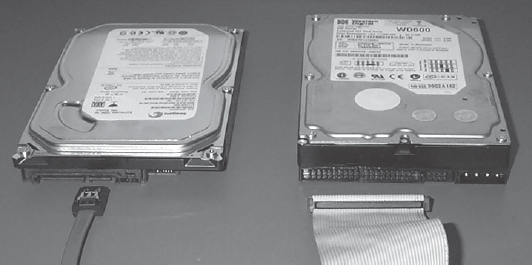
SATA The Serial ATA (SATA) interface is the successor to PATA. SATA drives use much slimmer cables than do PATA drives, as shown in Figure 4.2. Each SATA cable connects one device to the motherboard or SATA controller card, obviating the need for jumper configuration related to the drive identification. (Some SATA drives have jumpers for other purposes, though.) Although most SATA devices are internal to the computer, an external variant of the protocol, known as eSATA, is used by some external drives.
FIGURE 4.2 SATA (left) features much slimmer connecting cables than the older PATA (right).
SCSI The Small Computer System Interface (SCSI) standard physically resembles PATA, in that it uses ribbon cables, although they're slightly wider, with 50 pins. SCSI supports up to 8 or 16 devices per cable, depending on the SCSI version, but the SCSI host adapter in the computer counts as a device, so the limit on the number of disks is seven or fifteen. In the past, SCSI was the favorite for servers and high-end workstations. Today, SCSI has faded in popularity, but SCSI devices are still available. A next-generation SCSI interface, known as Serial Attached SCSI (SAS), is also available. In addition to being the next-generation SCSI interface, SAS is a step toward integrating the SCSI and ATA lines.
USB The Universal Serial Bus is a popular method of interfacing external devices, including portable hard disks and USB flash drives. The first and second generations of USB are poor performers compared to all but rather elderly dedicated hard disk interfaces, but USB 3.0 greatly improves USB speed.
In addition to these four interfaces, various others are or have been used. These alternative interfaces are either modern but rare (such as IEEE-1394, aka FireWire) or obsolete interfaces.
From a Linux software perspective, all but the most obscure hard disk hardware uses one of two driver sets:
PATA The PATA drivers, identified in the kernel as ATA/ATAPI/MFM/RLL, are officially deprecated with the most recent kernels, meaning that these drivers are still supported but are likely to be removed in the future. These drivers are most often used with PATA disks; however, this driver set includes support for some SATA hardware. Devices using these drivers receive names of the form /dev/hda, /dev/hdb, and so on. The first of these (/dev/hda) is reserved for the master drive on the first controller, /dev/hdb is the slave drive on the first controller, /dev/hdc is the master drive on the second controller, and so on. Thus, depending on how drives are connected, letters may be skipped—a computer can have /dev/hda and /dev/hdc but not /dev/hdb. PATA optical drives receive the same types of identifiers, although they can also usually be accessed as /dev/cdrom and other similar names.
SCSI The Linux kernel's SCSI subsystem, originally used by SCSI devices, has slowly adopted other disk device types, including most SATA devices, USB devices, and today even many PATA devices. Hard disks managed by Linux's SCSI drivers receive names of /dev/sda, /dev/sdb, and so on. Gaps in the sequence don't normally exist for internal hard disks, but they can develop when USB or other external disks are removed. Optical disks managed by these drivers use names of /dev/sr0, /dev/sr1, and so on, with symbolic links using /dev/cdrom, /dev/dvd, and similar names.
It's important to realize that Linux's disk drivers are written for the controller circuitry on the motherboard or disk controller card; individual disks need no driver per se, since disk hardware is standardized within each category. The techniques and utilities described in the next few pages, however, enable you to tweak disk access methods in case a particular disk's needs aren't properly auto-detected.
Most modern computers include connectors for at least four disk devices on the motherboard. In most cases, the motherboard's main chipset provides the disk controller circuitry. In some cases, particularly on motherboards that support more than four disks, two different disk controllers are used. Plug-in cards are available to expand the number or type of disk devices a computer can use.
![]() In some cases, connecting a disk to a different motherboard controller port can overcome performance problems. This can be true if switching ports moves the disk from one disk controller to another one; sometimes the Linux drivers for one controller are deficient, or there may be disk/controller hardware incompatibilities that impede performance. Such a swap is usually easy to implement once you've opened the computer's case, so it can be a good thing to try if you're having disk problems.
In some cases, connecting a disk to a different motherboard controller port can overcome performance problems. This can be true if switching ports moves the disk from one disk controller to another one; sometimes the Linux drivers for one controller are deficient, or there may be disk/controller hardware incompatibilities that impede performance. Such a swap is usually easy to implement once you've opened the computer's case, so it can be a good thing to try if you're having disk problems.
From a Linux configuration perspective, the nature of the technology used to store data—spinning platters on a hard disk, magneto-optical (MO) devices, solid state device (SSD) hardware, or something else—is mostly irrelevant. Such devices all present the same type of interface to Linux, using the PATA or SCSI drivers to enable the kernel and higher-level tools to read and write data from and to the disk. Some devices have subtle quirks, such as a need to align partitions in particular ways (as described in the Real World Scenario “Software vs. Hardware RAID”), but fundamentally they're the same. Optical drives (CD-ROMs, DVDs, and Blu-ray discs) are an exception; as described in Chapter 3, these devices must be accessed in different ways, particularly for writing.
Identifying Disk Resource Use
Disk controllers, like all hardware devices, use hardware resources. For the most part, resource use is managed automatically by the Linux kernel and its drivers; however, you may want to check on, and perhaps adjust, some details.
One important hardware resource is the interrupt request (IRQ, or interrupt) used by the device. Whenever some event occurs in the hardware device, such as the user pressing an eject button on a removable disk, the hardware signals this event to the computer via an interrupt. The traditional x86 architecture supports 16 interrupts, numbered 0–15; however, modern computers support more interrupts than this.
In the traditional x86 scheme, IRQs 14 and 15 are dedicated to the primary and secondary PATA controllers. Today, though, these interrupts might not be used. You can learn how your interrupts are allocated by examining the /proc/interrupts pseudo-file:
Scan the output's last column for a driver related to disk access. In this example, IRQs 16 and 19 are both associated with hda_intel, a disk driver; and IRQ 22 is linked with ahci, a modern disk-access method. IRQs 16 and 19 in this example are shared—multiple devices use the same interrupt. This seldom causes problems on modern hardware, but if you suspect your disk accesses are being impaired by a shared interrupt, you can look into driver module options to change how interrupts are assigned. Research the drivers for both your disk devices and whatever is sharing the interrupts with them, as described in Chapter 2. You can also review your computer's firmware options; these may enable you to adjust IRQ assignment. Finally, the sysctl utility and its configuration file, /etc/sysctl.conf, can often be used to adjust IRQ assignments. Try typing sysctl -a | grep irq to learn about relevant options and then change any you find in /etc/sysctl.conf.
A second type of hardware resource you might want to adjust is direct memory access (DMA) allocation. In a DMA configuration, a device transfers data directly to and from an area of memory, as opposed to passing data through the computer's CPU. DMA can speed access, but if two devices try to use the same DMA channel, data can be corrupted. You can examine /proc/dma to review DMA address assignments:
$ cat /proc/dma
 3: parport0
 4: cascade
DMA problems are extremely rare on modern computers. If you need to adjust them, though, you can review your driver documentation and sysctl settings much as you would for IRQ conflicts to find a way to reassign a device to use a new DMA channel.
Testing Disk Performance
If you suspect disk problems, you should first try to quantify the nature of the problem. The hdparm utility can be useful for this. Pass it the -t parameter to test uncached read performance on the device:
# hdparm -t /dev/sda

/dev/sda:
 Timing buffered disk reads: 264 MB in 3.00 seconds = 87.96 MB/sec
![]() Using an uppercase -T instead of a lowercase -t tests the performance of the disk cache, which is mostly a measure of your computer's memory performance. Although this measure isn't very interesting in terms of real disk performance, many people habitually do both tests at the same time, as in hdparm -tT /dev/sda. For best results, run the hdparm test two or three times on an unloaded system.
Using an uppercase -T instead of a lowercase -t tests the performance of the disk cache, which is mostly a measure of your computer's memory performance. Although this measure isn't very interesting in terms of real disk performance, many people habitually do both tests at the same time, as in hdparm -tT /dev/sda. For best results, run the hdparm test two or three times on an unloaded system.
As a general rule, conventional disks in 2011 should produce performance figures in the very high tens of megabytes per second and above. You can try to track down specifications on your disk from the manufacturer; however, disk manufacturers like to quote their disk interface speeds, which are invariably higher than their platter transfer rates (aka their internal transfer rates). Even if you can find an internal transfer rate for a drive, it's likely to be a bit optimistic.
SSD performance can be significantly better than that of conventional spinning disks, at least when using a true disk interface such as SATA. (USB flash drives tend to be quite slow.) If you apply hdparm to a RAID 0, 4, 5, 6, or 10 array, you're likely to see very good transfer rates, too.
Be aware that performance in actual use is likely to be lower than that produced by hdparm; this utility reads a large chunk of data from the drive without using the filesystem. In real-world use, the filesystem will be involved, which will degrade performance because of extra CPU overhead, the need to seek to various locations to read filesystem data, and other factors. Write performance may also be lower than read performance.
Adjusting Disk Parameters
If you use a device via a Linux PATA driver, the hdparm utility can be used to tweak disk access parameters, not just to measure performance. Table 4.7 summarizes the most important performance-enhancing features of hdparm, including one for power saving. Consult the program's man page for more hdparm options.
TABLE 4.7 hdparm options for enhancing performance
| Option | Explanation |
| -dn | PATA devices can be run in either Programmed Input/Output (PIO) mode or in DMA mode. DMA mode produces lower CPU loads for disk accesses. Using -d0 enables PIO mode, and -d1 enables DMA mode. The -d1 option is generally used in conjunction with -X (described shortly). This option doesn't work on all systems; Linux requires explicit support for the DMA mode of a specific ATA chipset if you're to use this feature. |
| -p mode | This parameter sets the PIO mode, which in most cases varies from 0 to 5. Higher PIO modes correspond to better performance. |
| -c mode | Queries or sets 32-bit transfer status. Omit mode to query the status, set mode to 0 to disable 32-bit support, set mode to 1 to enable 32-bit support, or set mode to 3 to enable 32-bit support using a special sequence needed by some chipsets. |
| -S timeout | This option sets an energy-saving feature: the time a drive will wait without any accesses before it enters a low-power state. It takes a few seconds for a drive to recover from such a state, so many desktops leave timeout at 0, which disables this feature. On laptops, though, you may want to set timeout to something else. Values between 1 and 240 are multiples of 5 seconds (for instance, 120 means a 600-0second, or 10-minute, delay); 241–251 mean 1–11 units of 30 minutes; 252 is a 21-minute timeout; 253 is a drive-specific timeout; and 255 is a 21-minute and 15-second timeout. |
| -v | You can see assorted disk settings with this option. |
| -Xtransfermode | This option sets the DMA transfer mode used by a disk. The transfermode is usually set to a value of sdmax, mdmax, or udmax. These values set simple DMA, multiword DMA, or Ultra DMA modes, respectively. In all cases, x represents the DMA mode value, which is a number. On modern hardware, you should be able to use a fairly high Ultra DMA mode, such as -X udma5 or -X udma6 . Use this option with caution; setting an improper mode can cause the disk to become inaccessible, which in turn can cause your system to hang. |
Although hdparm is useful for tuning PATA disks, most of its options have no effect on SCSI disks, including most SATA, USB, and even PATA disks that use the new SCSI interface for PATA. Fortunately, this isn't usually a problem, since true SCSI disks and the newer devices that are managed through the SCSI subsystem are generally configured optimally by default.
The sdparm utility, despite the name's similarity to hdparm, isn't really a SCSI equivalent of hdparm. Nonetheless, you can use sdparm to learn about and even adjust your SCSI devices. Table 4.8 summarizes the most important sdparm options; consult its man page for more obscure sdparm options. To use it, pass one or more options followed by a device name, such as /dev/sr0 or /dev/sda.
TABLE 4.8 Common sdparm options

![]() Many sdparm features enable sending low-level SCSI signals to your SCSI devices. This ability is potentially very dangerous. You should not experiment with random sdparm options.
Many sdparm features enable sending low-level SCSI signals to your SCSI devices. This ability is potentially very dangerous. You should not experiment with random sdparm options.
Monitoring a Disk for Failure
Modern hard disks provide a feature known as Self-Monitoring, Analysis, and Reporting Technology (SMART), which is a self-diagnostic tool that you can use to predict impending failure. Periodically checking your drives for such problems can help you avoid costly incidents; if a SMART tool turns up a problem, you can replace the disk before you lose any data!
Several SMART-monitoring tools for Linux are available. One of these is smartctl; you can obtain a SMART report on a drive by typing smartctl -a /dev/sda, where /dev/sda is the disk device node. Much of the output will be difficult to interpret, but you can search for the following line:
SMART overall-health self-assessment test result: PASSED
![]() The smartctl output is wider than the standard 80 columns. You'll find it easier to interpret if you run it from a console that's at least 90 columns wide. If you run it from an X-based terminal, widen it before you run smartctl.
The smartctl output is wider than the standard 80 columns. You'll find it easier to interpret if you run it from a console that's at least 90 columns wide. If you run it from an X-based terminal, widen it before you run smartctl.
Of course, if the report indicates a failure, you should peruse the remainder of the report to learn what the problem is. You can also use smartctl to run active tests on a drive; consult its man page for details.
If you prefer a GUI tool, the GSmartControl utility (http://gsmartcontrol.berlios.de) may be what you need. Launch it, click an icon corresponding to a hard disk, and you'll see a window similar to the one in Figure 4.3. The final summary line on the Identity tab reveals the drive's overall health. If that line indicates problems or if you want to peruse the details, you can click the other tabs. The Perform Tests tab enables you to run active tests on the drive.
FIGURE 4.3 A SMART monitoring tool enables you to identify failing disk hardware before it causes you grief.

If a SMART test reveals problems, you should replace the drive immediately. You can transfer data by partitioning the new disk and creating filesystems on it and then using tar or cpio to copy data, or you can use a backup and data transfer tool such as CloneZilla (http://clonezilla.org).
Backing Up and Restoring a Computer
Many things can go wrong on a computer that might cause it to lose data. Hard disks can fail, you might accidentally enter some extremely destructive command, a cracker might break into your system, or a user might accidentally delete a file, to name just a few possibilities. To protect against such problems, it's important that you maintain good backups of the computer. To do this, select appropriate backup hardware, choose a backup program, and implement backups on a regular schedule. You should also have a plan in place to recover some or all of your data should the need arise.
Choosing Backup Hardware
Just about any device that can store computer data and read it back can be used as a backup medium. The best backup devices are inexpensive, fast, high in capacity, and reliable. They don't usually need to be random-access devices, though. Random-access devices are capable of quickly accessing any piece of data. Hard disks, CD-ROMs, and DVDs are all random-access devices. These devices contrast with sequential-access devices, which must read through all intervening data before accessing the sought-after component. Tapes are the most common sequential-access devices. Table 4.9 summarizes critical information about the most common types of backup device. For some such as tape, there are higher-capacity (and more expensive) devices for network backups.
TABLE 4.9 Vital statistics for common backup devices
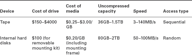
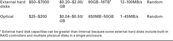
Numbers are approximate as of late 2010. Prices on all storage media have historically fallen rapidly, and capacities have risen. Costs are likely to be lower, and capacities higher, in the future.
The types of devices that appear in Table 4.9 are those most often used for backing up Linux systems. The pros and cons of using specific devices are:
Tapes Tape drives have historically been the most popular choice for backing up entire computers. Their sequential-access nature is a hindrance for some applications, but it isn't a problem for routine backups. The biggest problem with tapes is that they're less reliable than some backup media, although reliability varies substantially from one type of tape to another, and the best are reasonably reliable.
Hard Disks It's possible to use hard disks for backup purposes. If your computer is equipped with a kit that enables a drive to be quickly removed from a computer, you can swap hard disks in and out and move them off-site for storage, if desired. Similar comments apply to external hard disks. Internal hard disks without a removable disk bay, however, are susceptible to theft or damage along with the computer they're meant to back up.
Optical Optical media are reliable in the short term, but less reliable in the long term than once believed. High-quality media, properly stored, can theoretically last decades; but in practice, failures sometimes occur after only a year or two. Some optical media are large enough to back up entire small systems, but for really large jobs, the higher capacity of tapes or hard disks is desirable. The need to use special tools, such as cdrecord, to write to optical devices can complicate backup plans, but this isn't an insurmountable hurdle.
In the past, the best backup devices for entire computers and networks have been tapes. The low cost and high capacity of tapes made them well suited to performing multiple backups of entire computers. In recent years, though, hard disks have plummeted in price, making removable or external hard disks more appealing than tapes for many applications. It's sometimes desirable to supplement tape or removable hard disk backups with optical backups.
It's generally wise to keep multiple backups and to store some of them away from the computers they're meant to protect. Such off-site storage protects your data in case of fire, vandalism, or other major physical traumas. Keeping several backups makes it more likely you'll be able to recover something, even if it's an older backup, should your most recent backup medium fail. Some administrators like to follow the 3-2-1 strategy for backups, which involves keeping three copies of the data on at least two different types of media with at least one copy off-site.
Tape devices are accessed in Linux using the /dev/st0 (SCSI) or /dev/ht0 (PATA) device filenames. The /dev/nst0 and /dev/nht0 filenames are non-rewinding variants of these names—when using /dev/st0 or /dev/ht0, the tape rewinds automatically after every operation; but when using /dev/nst0 or /dev/nht0, the tape does not rewind. If a computer has more than one tape drive of a particular type, the number at the end of the device filename is incremented for each additional drive, as in /dev/st1 for the second SCSI tape drive.
If you decide to use hard disks in removable mounts as a backup medium, you'll need ordinary internal drives and mounting hardware. The hardware comes in two parts: a mounting bay that fits in the computer and a frame in which you mount the hard drive. To use the system, you slide the frame with hard drive into the mounting bay. You can get by with one of each component, but it's best to buy one frame for each hard drive, which effectively raises the media cost. From a Linux software point of view, removable hard disk systems work like regular hard disks or other removable disk systems, like USB flash drives. Most of these systems use SATA disks, which you'll access as /dev/sdb, /dev/sdc, or some other SCSI device identifier. The disks are likely to be partitioned, and the partitions are likely to hold ordinary Linux filesystems.
External disks with USB or eSATA interfaces are very common and can make good backup media; however, you'll need to buy several of them for optimum backup security. Alternatively, you can use an external caddy or cable, to which you can easily attach a bare hard disk. Buying one caddy and several hard disks enables you to keep multiple backups. For optimum speed, get a USB 3.0 or eSATA drive—and be sure your computer supports this high-performance interface!
Choosing Backup Software
Linux supports several backup programs. Some are tools designed to back up individual files, directories, or computers. Others build on these simpler tools to provide network backup facilities. Basic backup programs include tar, cpio, dump, and dd. ARKEIA (http://www.arkeia.com) and BRU (http://www.tolisgroup.com) are two commercial backup packages that provide explicit network support and GUI front-ends. AMANDA (http://www.amanda.org), Bacula (http://www.bacula.org), and BackupPC (http://backuppc.sourceforge.net) are network-capable backup packages that can perform a backup of an entire network. The rsync utility is a relatively simple program for performing network data transfers. When dealing with tapes, the mt program is useful for controlling the tape hardware.
This section provides a look at tar, cpio, dd, rsync, and mt as examples of how to back up a Linux system.
Using tar
The tar program's name stands for “tape archiver.” Despite this, you can use tar to archive data to other media. In fact, tarballs (archive files created by tar and typically compressed with gzip or bzip2) are often used for transferring multiple files between computers in one step, such as when distributing source code. (Chapter 1 describes the use of tar in this context.)
The tar program is a complex package with many options, but most of what you'll do with the utility can be covered with a few common commands. Table 4.10 lists the primary tar commands, and Table 4.11 lists the qualifiers that modify what the commands do. Whenever you run tar, you use exactly one command, and you usually use at least one qualifier.
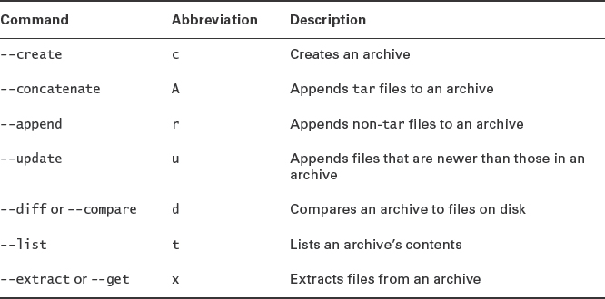


Of the commands listed in Table 4.10, the most commonly used are --create, --extract, and --list. The most useful qualifiers from Table 4.11 are --file, --listed-incremental, --one-file-system, --same-permissions, --gzip, --bzip2, and --verbose. If you fail to specify a filename with the --file qualifier, tar will attempt to use a default device, which is often (but not always) a tape device file.
Using cpio
The cpio program is similar to tar in that it creates an archive file. That file can be stored on disk, or it can be directed straight to your tape device. This can be a convenient way to back up the computer, because it requires no intermediate storage. To restore data, you use cpio to read directly from the tape device file.
The cpio utility has three operating modes:
Copy-Out Mode This mode, activated by use of the -o or --create option, creates an archive and copies files into it.
Copy-In Mode You activate copy-in mode by using the -i or --extract option. This mode extracts data from an existing archive. If you provide a filename or a pattern to match, cpio will extract only the files whose names match the pattern you provide.
Copy-Pass Mode This mode is activated by the -p or --pass-through option. It combines the copy-out and copy-in modes, enabling you to copy a directory tree from one location to another.
![]() The copy-out and copy-in modes are named confusingly.
The copy-out and copy-in modes are named confusingly.
In addition to the options used to select the mode, cpio accepts many other options, the most important of which are summarized in Table 4.12. To back up a computer, you'll combine the --create (or -o) option with one or more of the options in Table 4.12; to restore data, you'll do the same but use --extract (or -i). In either case, cpio acts on filenames that you type at the console. In practice, you'll probably use the redirection operator (<) to pass a filename list to the program.
TABLE 4.12 Options for use with cpio
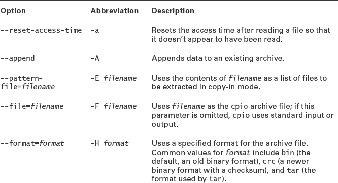
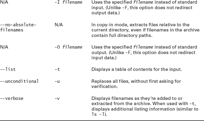
Using dd
The dd utility is a low-level file copying tool, with the ability to apply certain transformations at the same time. As a backup tool, dd is useful for backing up an entire raw filesystem—even one that Linux doesn't support or one that's been badly damaged. Table 4.13 summarizes the dd options you're most likely to use when backing up a filesystem using this tool. Consult the program's man page for additional options.
To use dd to back up a partition, you specify the original partition's device filename with if= and a backup partition, file, or device with of=. For instance, if you want to back up /dev/sda2 to a file on an external hard disk that's mounted at /media/backups, you might type the following:
# dd if=/dev/sda2 of=/media/backups/sda2-back.img
If you wanted to restore the backup, you would reverse the if= and of= operands.
![]() You should back up or restore only unmounted filesystems using dd. Backing up a mounted filesystem can produce an inconsistent filesystem. Restoring to a mounted partition can produce severe disk corruption. If you need to back up a running system using dd and if the device in question is part of an LVM, you can use the LVM snapshot feature, as described earlier in “Using LVM Snapshots,” and back up the snapshot volume.
You should back up or restore only unmounted filesystems using dd. Backing up a mounted filesystem can produce an inconsistent filesystem. Restoring to a mounted partition can produce severe disk corruption. If you need to back up a running system using dd and if the device in question is part of an LVM, you can use the LVM snapshot feature, as described earlier in “Using LVM Snapshots,” and back up the snapshot volume.
If you want to apply compression, you can omit the of= (on backup) or if= (on restore) option and use dd with a compression program in a pipe:
# dd if=/dev/sda2 | gzip -9 > /media/backups/sda2-back.img.gz
# gunzip /media/backups/sda2-back.img.gz - | dd of=/dev/sda2
The first command backs up /dev/sda2; the second command restores that partition.
The greatest strength of dd is its filesystem independence; you can back up anything with dd, even if Linux provides limited or no support for the filesystem. You can also back up a damaged filesystem with dd, which is useful if you want to attempt a repair but fear causing further damage to the original filesystem. The biggest problem with dd is that, because it backs up everything on a byte-by-byte basis, it wastes time and disk space backing up unused space in the filesystem. If you have a 20 GiB partition, it will take 20 GiB of backup storage space if backed up uncompressed, even if the partition holds just 2 KiB of files. Applying compression can minimize this problem, but in some cases, unused parts of a filesystem actually hold old data, so the backup can still be larger than necessary.
![]() The dcfldd utility (http://dcfldd.sourceforge.net) is a dd variant with additional features, such as a progress indicator. The ddrescue utility (http://www.gnu.org/software/ddrescue/ddrescue.html), although dissimilar from dd and dcfldd in usage details, tries extra hard to recover data from bad media, which is sometimes vitally important.
The dcfldd utility (http://dcfldd.sourceforge.net) is a dd variant with additional features, such as a progress indicator. The ddrescue utility (http://www.gnu.org/software/ddrescue/ddrescue.html), although dissimilar from dd and dcfldd in usage details, tries extra hard to recover data from bad media, which is sometimes vitally important.
Using rsync
For small network backup tasks, rsync may be all you need. This program is designed to copy data from one computer to another on a network, keeping two network directories synchronized. The program supports a large number of options and variant machine specifications; however, a general use looks something like this:
$ rsync -av ./ user@remote:~/backups/
This command copies all the files in the current directory to the remote computer, using the username user, and places the files in the ~/backups directory on that system.
As shown here, rsync can be used by ordinary users. Alternatively, it can be used by a backup script to do its transfers. In either case, rsync relies on another network file-transfer tool, such as ssh. In some cases, this tool may require a password, so you may need to be present to type it; or you can configure the computers to enable password-free file transfers.
Although rsync doesn't transfer data directly to a backup medium unless it's a hard disk that's mounted, it can be useful for network data transfers. Users can copy their files to a central backup server, or the backup server can use rsync to grab files from backup client computers. In either case, the backup server computer can then back the files up to tape or some other storage medium.
Using cpio or tar to Back Up a Computer
The preceding sections describe the basic features of several common backup utilities. It is informative to see how these tools are used in practice, though. Therefore, this section illustrates how to use cpio or tar to back up a computer.
It's often desirable to compress backups, but the cpio and tar programs don't compress data themselves. To do this, these programs rely on an external program, such as gzip or bzip2, to compress an entire cpio or tar archive. The problem with this approach is that if an error occurs while restoring the compressed archive, all the data from that error onward will be lost. This makes compressed cpio or tar archives risky for backup. Fortunately, most tape drives support compression in their hardware, and these use more robust compression algorithms. Therefore, if your tape drive supports compression, you should not compress a cpio or tar backup. Let the tape drive do that job, and if there's a read error at restore, you'll probably lose just one or two files. If your tape drive doesn't include built-in compression features, you should either not compress your backups or use another utility, most of which don't suffer from this problem.
To back up a computer with cpio, a command like the following will do the job:
# find / | cpio -oF /dev/st0
Because cpio expects a list of files on standard input, this command uses the find command and a pipe to feed this information to cpio. The -o option then tells cpio to create an archive, and -F specifies where it should be created—in this case, it uses /dev/st0 to create the archive on the tape device.
This command, though, has some negative effects. Most notably, it backs up everything, including the contents of the /proc filesystem and any mounted removable disks that might be present. You can use the -xdev option to find to have that program omit mounted directories from its search, but this means you'll have to explicitly list each partition you want to have backed up. For instance, you might use a command like the following to back up the /home, root (/), /boot, and /var partitions:
# find /home / /boot /var -xdev | cpio -oF /dev/st0
![]() This command lists directories in a particular order. Because tape is a sequential-access medium, the system will restore items in the order in which they were backed up. Therefore, for the fastest partial restores, list the filesystems that you most expect to have to restore first. In this example, /home is listed first because users sometimes delete files accidentally. Backing up /home first, therefore, results in quicker restoration of such files.
This command lists directories in a particular order. Because tape is a sequential-access medium, the system will restore items in the order in which they were backed up. Therefore, for the fastest partial restores, list the filesystems that you most expect to have to restore first. In this example, /home is listed first because users sometimes delete files accidentally. Backing up /home first, therefore, results in quicker restoration of such files.
Depending on the filesystem you use, you may see a string of truncating inode number messages. This happens when you use an old cpio format with a filesystem that uses inode numbers greater than 65,536. To overcome this problem, specify another format, such as crc, using -H.
The procedure for backing up with tar is similar; however, tar doesn't need a list of files piped to it; you provide a list of files or directories on the command line:
# tar cvpf /dev/st0 --one-file-system /home / /boot /var
Ordinarily, tar descends the directory tree; the --one-file-system option prevents this, much like the -xdev option to find.
After creating a backup with tar, you may want to use the tar --diff (also known as --compare, or d) command to verify the backup you've just written against the files on disk. Alternatively, you can include the --verify (W) qualifier to have this done automatically. Verifying your backup doesn't guarantee it will be readable when you need it, but it should at least catch major errors caused by severely degraded tapes. On the other hand, the verification will almost certainly return a few spurious errors because of files whose contents have legitimately changed between being written and being compared. This may be true of log files, for instance.
Backing Up Using Optical Media
Optical media require special backup procedures. As described in Chapter 3, tools such as cdrecord or growisofs are required to write to these discs.
One option for backing up to optical discs is to use mkisofs and then cdrecord to copy files to a CD-R or use growisofs to copy files to a DVD or Blu-ray disc. If you copy files “raw” in this way, though, you'll lose some information, such as write permission bits. You'll have better luck if you create a cpio or tar file on disk, much as you would when you back up to tape. You would then use mkisofs/cdrecord or growisofs to copy this file to the disc. The result will be a CD-R that you can mount and that will contain an archive you can read with cpio or tar.
A somewhat more direct option is to create an archive file and burn it directly to the optical disc using cdrecord, bypassing mkisofs. Such a disc won't be mountable in the usual way, but you can access the archive directly by using the optical device file. On restoration, this works much like a tape restore, except that you specify the optical device filename (such as /dev/cdrom) instead of the tape device filename (such as /dev/st0).
Using mt to Control a Tape Drive
In cpio and tar terminology, each backup is a file. This file is likely to contain many files from the original system, but like an RPM or Debian package file, the archive file is a single entity. Sometimes an archive file is far smaller than the tape on which it's placed. If you want to store more than one archive file on a tape, you can do so by using the nonrewinding tape device filename. For instance, the following commands accomplish the same goal as the ones shown in the previous section, but in a somewhat different manner and with subtly different results:
# tar cvlpf /dev/nst0 /home
# tar cvlpf /dev/nst0 /
# tar cvlpf /dev/nst0 /boot
# tar cvlpf /dev/nst0 /var
After you issue these commands, the tape will contain four tar files, one for each of the four directories. To access each file after writing them, you need to use a special utility called mt. This program moves forward and backward among tape files and otherwise controls tape features. Its syntax is as follows:
mt -f device operation [count] [arguments]
The device parameter is the tape device filename. The mt utility supports many operations, as summarized in Table 4.14.
TABLE 4.14 Common mt operations
| Operation | Description |
| fsf | Moves forward count files. |
| bsf | Moves backward count files. |
| eod or seod | Moves to the end of data on the tape. |
| rewind | Rewinds the tape. |
| offline or rewoffl | Rewinds and unloads the tape. (Unloading is meaningless on some drives but ejects the tape on others.) |
| retension | Rewinds the tape, winds it to the end, and then rewinds it again. This action improves reliability with some types of tape, particularly if the tape has been sitting unused for several months. |
| erase | Erases the tape. (This command usually doesn't actually erase the data; it just marks the tape as being empty.) |
| status | Displays information on the tape drive. |
| load | Loads a tape into the drive. Unnecessary with many drives. |
| compression | Enables or disables compression by passing an argument of 1 or 0, respectively. |
| datcompression | Also enables and disables compression. |
![]() The compression and datcompression operations aren't identical; sometimes a tape drive works with one but not the other.
The compression and datcompression operations aren't identical; sometimes a tape drive works with one but not the other.
For instance, suppose you created a backup on a SCSI tape, but now you want to create another backup on the same tape without eliminating the first backup. You could issue the following commands to accomplish this task:
# mt -f /dev/nst0 rewind
# mt -f /dev/nst0 fsf 1
# tar cvlpf /dev/nst0 /directory/to/back/up
# mt -f /dev/nst0 offline
These commands rewind the tape, space past the first file, create a new backup, and then unload the tape. Such commands are particularly useful when performing incremental backups, as described shortly.
Planning a Backup Schedule
Regular computer backup is important, but precisely how regularly is a matter that varies from one system to another. If a computer's contents almost never change (as might be true of a dedicated router or a workstation whose user files reside on a file server), backups once a month or even less often might be in order. For critical file servers, once a day is not too often. You'll have to decide for yourself just how frequently your systems require backup. Take into consideration factors such as how often the data change, the importance of the data, the cost of recovering the data without a current backup, and the cost of making a backup. Costs may be measured in money, your own time, users' lost productivity, and perhaps lost sales.
Even the most zealous backup advocate must admit that creating a full backup of a big system on a regular basis can be a tedious chore. A backup can easily take several hours, depending on backup size and hardware speed. For this reason, most backup packages, including tar, support incremental backups. You can create these using the --listed-incremental file qualifier to tar, as shown in this example:
# tar cvplf /dev/st0 --listed-incremental /root/inc / /home
This command stores a list of the files that have been backed up (along with identifying information to help tar determine when the files have changed) in /root/inc. The next time the same command is issued, tar will not back up files that have already been backed up; it will back up only new files. Thus, you can create a schedule in which you do a full backup of the entire computer only occasionally—say, once a week or once a month. You'd do this by deleting the increment file and running a backup as usual. On intervening weeks or days, you can perform an incremental backup, in which only new and changed files are backed up. These incremental backups will take comparatively little time.
With cpio, the key to incremental backups is in the list of files fed to the program. You can perform an incremental backup by using find options to locate only new files or files that have changed since the last backup. For instance, the -newer file option to find causes that program to return only files that have been modified more recently than file. Thus, you could create a file (perhaps a log of your backup activity) during each backup and use it as a way of determining what files have been modified since the last backup.
You can use incremental backups in conjunction with mt to store multiple incremental backups on one tape. Typically, you'll have two tapes for a backup set: one for a full backup and one for intervening incremental backups. Suppose you do a full backup on Monday. On Tuesday, you'd insert the incremental tape and perform the first incremental backup. On Wednesday, you'd insert this tape and type mt -f /dev/nst0 fsf 1 to skip past Tuesday's incremental backup, and then perform another incremental backup. On Thursday, you'd type mt -f /dev/nst0 fsf 2, and so on.
Performing incremental backups has a couple of drawbacks. One is that they complicate restoration. Suppose you do a full backup on Monday and incremental backups every other day. If a system fails on Friday, you'll need to restore the full backup and several incremental backups. Second, after restoring an incremental backup, your system will contain files that you'd deleted since the full backup. If files have short life spans on a computer, this can result in a lot of “dead” files being restored when the time comes to do so.
Despite these problems, incremental backups can be an extremely useful tool for helping make backups manageable. They can also reduce wear and tear on tapes and tape drives, and they can minimize the time it takes to restore files if you know that the files you need to restore were backed up on an incremental tape.
![]() Whether you perform incremental backups or nothing but complete backups, you should maintain multiple backups. Murphy's Law guarantees that your backup will fail when you need it most, so having a backup for your backup (even if it's from a week or a month earlier) can help immensely. A typical backup plan includes a rotating set of backup tapes. For instance, you might have two tapes per week—one for a full backup on one day and one to hold several incremental backups. Eight tapes will then hold backups for four weeks.
Whether you perform incremental backups or nothing but complete backups, you should maintain multiple backups. Murphy's Law guarantees that your backup will fail when you need it most, so having a backup for your backup (even if it's from a week or a month earlier) can help immensely. A typical backup plan includes a rotating set of backup tapes. For instance, you might have two tapes per week—one for a full backup on one day and one to hold several incremental backups. Eight tapes will then hold backups for four weeks.
Preparing for Disaster: Backup Recovery
Creating backups is advisable, but doing this isn't enough. You must also have some way to restore backups in case of disaster. This task involves two aspects: partial restores and emergency recovery.
Partial restores involve recovering just a few noncritical files. For instance, users might come to you and ask you to restore files from their home directories. You can do so fairly easily by using the --extract (x) tar command, as in:
# cd /
# tar xvpf /dev/st0 home/username/filename
![]() This sequence involves changing to the root directory and issuing a relative path to the file or directory that must be restored. This is required because tar normally strips away the leading / in files it backs up, so the files are recorded in the archive as relative filenames. If you try to restore a file with an absolute filename, it won't work.
This sequence involves changing to the root directory and issuing a relative path to the file or directory that must be restored. This is required because tar normally strips away the leading / in files it backs up, so the files are recorded in the archive as relative filenames. If you try to restore a file with an absolute filename, it won't work.
When you're using cpio, the procedure is similar, but you use the --extract (-i) option, along with other options to feed the name of the archive, and perhaps do other things:
# cd /
# cpio -ivF /dev/st0 home/username/filename
![]() This cpio command uses -F to have cpio retrieve data from the specified file (/dev/st0) rather than from standard input. Alternatively, you could use redirection to do the job, as in cpio -iv < /dev/st0 home/username/filename.
This cpio command uses -F to have cpio retrieve data from the specified file (/dev/st0) rather than from standard input. Alternatively, you could use redirection to do the job, as in cpio -iv < /dev/st0 home/username/filename.
Whether you're using tar or cpio, you'll need to know the exact name of the file or directory you want to restore in order to do this. If you don't know the exact filename, you may need to use the --list (t) command to cpio or tar to examine the entire contents of the tape, or at least everything until you see the file you want to restore.
![]() If you use incremental backups, you can use the incremental file list to locate the filename you want to restore.
If you use incremental backups, you can use the incremental file list to locate the filename you want to restore.
A much more serious problem is that of recovering a system that's badly damaged. If your hard disk has crashed or your system has been invaded by crackers, you must restore the entire system from scratch, without the benefit of your normal installation. You can take any of several approaches to this problem, including the following:
Distribution's Installation Disk Most Linux distributions' installation disks have some sort of emergency recovery system. These systems are typically small but functional Linux installations with a handful of vital tools, such as fdisk, mkfs, Vi, and tar. Check your distribution's documentation or boot its boot media and study its options to learn more.
CD-Based Linux System Several Linux systems are now available that boot from CD-ROM or DVD. Examples include Knoppix (http://www.knoppix.com), SystemRescueCd (http://www.sysresccd.org), and PartedMagic (http://partedmagic.com). All of these systems can be used to help recover or restore a corrupted Linux installation.
Emergency System on Removable Disk You can create your own emergency system on a removable disk, such as a USB flash drive. A 16 GiB flash drive is sufficient to hold a fairly comfortable Linux installation, although it won't perform as quickly as an installation on a PATA, SATA, or SCSI hard disk.
Emergency Recovery Partition If you plan ahead, you might create a small emergency installation of your preferred distribution alongside the regular installation. You should not mount this system in /etc/fstab. This system can be useful for recovering from some problems, such as software filesystem corruption, but it's not useful for others, such as a total hard disk failure.
Partial Reinstallation You can reinstall a minimal Linux system and then use it to recover your original installation. This approach is much like the emergency recovery partition approach, but it takes more time at disaster recovery. On the other hand, it will work even if your hard disk is completely destroyed.
Whatever approach you choose to use, you should test it before you need it. Learn at least the basics of the tools available in any system you plan to use. If you use unusual backup tools (such as commercial backup software), be sure to copy those tools to your emergency system or have them available on a separate removable disk. If you'll need to recover clients via network links, test those setups as well.
You may not be able to completely test your emergency restore tools. Ideally, you should boot the tools, restore a system, and test that the system works. This may be possible if you have spare hardware on which to experiment, but if you lack this luxury, you may have to make do with performing a test restore of a few files and testing an emergency boot procedure—say, using Super GRUB Disk (http://www.supergrubdisk.org). Note that a freshly restored system will not be bootable; you'll need a tool such as Super GRUB Disk to boot the first time. You can then reinstall GRUB to restore the system's ability to boot from the hard disk.
Summary
Most Linux distributions create fairly conventional partition-based installations by default; however, advanced tools can be very useful alternatives to conventional partitioning schemes in certain situations. RAID enables you to combine multiple hard disks together to create larger filesystems, to improve speed, to improve reliability, or to do all these things. LVM can use a single storage area or multiple storage areas to create larger filesystems, to improve speed, to improve flexibility, or to do all of these things. You can combine RAID and LVM to gain all of these benefits. Both RAID and LVM, however, come at the cost of added complexity, and some configurations can reduce reliability.
Tuning disk access can improve disk performance. The most dramatic improvements are possible with older PATA disks, particularly if the default drivers and options are misconfigured for the disks. For more modern SCSI and SATA disks, dramatic performance improvements are unlikely, but you may want to test your disk's performance just to be sure it's reasonable. This includes using a SMART utility to verify that the disk hardware isn't on the verge of failing.
After you put effort into creating an ideal partitioning, RAID, or LVM setup; installing Linux; and tweaking the system, it would be a shame to throw away all that effort. Your users would say the same about their data on your computer. Thus, you should plan and deploy a backup strategy, backing up your data on a regular basis. If you do so, problems such as major user error, major software bugs, system intrusions, hardware failure, and even hardware theft can be overcome in a matter of minutes or hours by restoring a backup.
Exam Essentials
Explain the partitioning needs of a RAID configuration. MBR partitions added to a Linux software RAID array must be of type 0xFD. On a GPT disk, the partition is flagged as type 0xFD00 in GPT fdisk or as having the raid flag set in libparted-based tools. A single disk may hold one or more RAID partitions, each of which is combined with a matched partition on another physical disk.
Summarize the major levels of RAID supported by Linux. Linear RAID, although technically not RAID, combines devices in a simple one-after-the-other manner. RAID 0 combines two equal-sized devices in an interleaved manner to improve performance. RAID 1 creates a duplicate copy of one device on another one to improve reliability. RAID levels 4, 5, and 6 use checksums and one (two for RAID 6) extra device to improve both reliability and speed. RAID 10 is similar to RAID 4 and 5 in purpose, but it works by combining RAID 1 and RAID 0 features.
Explain the partitioning needs of an LVM configuration. MBR partitions in a Linux LVM setup must be of type 0x8E. On a GPT disk, the partition is flagged as type 0x8E00 in GPT fdisk or as having the lvm flag set in libparted-based tools. A single disk may hold one or more LVM partitions, which can be combined together or with partitions on other disks to create a volume group.
Summarize the three levels of data structures employed by LVM. Physical volumes are at the bottom of the LVM data structure hierarchy; these are partitions, RAID volumes, or other low-level devices that are suitably flagged and marked with basic LVM data structures. Physical volumes are combined into volume groups, which act as a pool of allocatable disk space. Logical volumes are created within this pool of disk space and can be used much like partitions; they typically hold filesystems or swap space.
Describe how LVM can improve backup operations. You can create a snapshot of a logical volume—that is, a duplicate of the original logical volume that won't change even as accesses continue on the original. By backing up the snapshot rather than the original logical volume, you ensure that it will be in a consistent state, even if the original is being used heavily and therefore might yield a backup that contains slightly mismatched files.
Describe how PATA disk access speed can be optimized. You can use the hdparm program to test raw disk read speed and to set various low-level disk access options. These include the use of DMA versus PIO mode, as well as the specific DMA or PIO transfer mode. These options are meaningful only for older PATA disks using the recently deprecated PATA drivers.
Summarize common backup hardware options. Tape is the traditional backup medium, and it remains a good choice for large installations. Tape can be expensive for small systems, though. For such computers, a removable or external hard disk can be a good alternative. Optical media (CD-Rs, recordable DVDs, and recordable Blu-ray discs) can be a useful backup medium for smaller systems or for small amounts of data, but these media lack the capacity to back up very large installations.
Summarize common backup software options. The tar and cpio programs are both popular file-based backup tools that are useful for backing up complete Linux installations. When backing up exotic filesystems that Linux might not fully support or when you need a low-level image prior to attempting repairs or modifications of a valuable filesystem, dd is a good choice. Commercial and network-based tools, such as BRU, ARKEIA, AMDANDA, Bacula, and BackupPC, are useful for backing up large systems or for performing backups of entire networks.
Explain common backup schedules. A full backup backs up all the files on a computer or in a directory tree. Such backups are easy to restore but consume a great deal of space on the backup medium. To save time and space, incremental backups can be performed in between full backups. These backups store only the files that have changed since the last full or incremental backup. Typically, you'll perform a full backup every once in a while (perhaps once a month or once a week), with incremental backups more frequently. The optimum schedule depends on many factors, including how often your files change, how valuable your data are, and your available resources.
Review Questions
- Typing fdisk -lu /dev/hda on a Linux computer with an MBR disk produces a listing of four partitions: /dev/hda1, /dev/hda2, /dev/hda5, and /dev/hda6. Which of the following is true?
A. The disk contains two primary partitions and two extended partitions.
B. Either /dev/hda1 or /dev/hda2 is an extended partition.
C. The partition table is corrupted; there should be a /dev/hda3 and a /dev/hda4 before /dev/hda5.
D. If you add a /dev/hda3 with fdisk, /dev/hda5 will become /dev/hda6, and /dev/hda6 will become /dev/hda7.
- A new server is arriving at the end of the week. It will have four 1 TiB hard drives installed and configured in a RAID 5 array with no hot standby spare drives. How much data can be stored within this array?
A. 4 TiB
B. 3 TiB
C. 2 TiB
D. 1 TiB
- You have been told by your manager that the server being moved from the test lab to production must have the two drives within it mirrored. What level of RAID is used for mirroring?
A. RAID 6
B. RAID 5
C. RAID 1
D. RAID 0
- What can you conclude from the following line, which is found in /proc/mdstat?
md0 : active raid4 sdd2[2] sdc1[1] sda8[0]
A. The /dev/md0 RAID 4 device is built from the /dev/sda8, /dev/sdc1, and /dev/sdd2 partitions.
B. The /dev/md0 RAID device is missing one partition; it should have four component partitions, given its RAID level (4).
C. The /dev/md0 RAID device is badly misconfigured; the partition numbers of the component devices should match.
D. None of the above.
- Which of the following commands correctly assembles a RAID 1 array from the component devices /dev/sda1 and /dev/hda2?
A. mdadm --create --level=1 --raid-devices=2 /dev/sda1 /dev/hda2
B. mdadm --level=1 --raid-devices=2 /dev/sda1 /dev/hda2
C. mdadm --level=5 --raid-devices=2 /dev/sda1 /dev/hda2
D. mdadm --create /dev/md0 --level=1 --raid-devices=2 /dev/sda1 /dev/hda2
- Once Linux is booted, which file can you view to see which IRQs are in use on the Linux computer?
A. /etc/interrupts
B. /boot/interrupts
C. /root/interrupts
D. /proc/interrupts
- Why should you be cautious when using hdparm?
A. The hdparm tool can set hardware options that are not supported by some hardware, thus causing data corruption.
B. Because hdparm modifies partition tables, an error can result in loss of one or more partitions and all their data.
C. By changing hardware device file mappings, you can become confused about which drive is /dev/hda and which is /dev/hdb.
D. The hdparm tool can cause Linux to treat an ext2fs partition as if it were FAT, resulting in serious data corruption.
- Which of the following tools is used to initialize a partition so that it may function as a physical volume in an LVM configuration?
A. pvchange
B. pvcreate
C. lvcreate
D. lvconvert
- Which of the following device files might you reasonably include in a volume group, assuming they're properly flagged and prepared? (Select all that apply.)
A. /dev/sdc
B. /dev/md1
C. /dev/sda7
D. /dev/hdb2
- Your computer has crashed because of filesystem corruption, and you must perform emergency recovery using an emergency boot disc. How can you activate your LVM devices, if they aren't activated automatically when you boot your emergency disc?
A. vgscan
B. vgimport
C. vgchange -ay
D. vgdisplay
- Where are you likely to find device nodes for the MyGroup volume group?
A. /dev/mapper
B. /dev/mygroup
C. /dev/lvm
D. /dev/LVM/MyGroup
- What is the appropriate procedure for increasing the size of a logical volume containing an ext3 filesystem? (Assume sufficient free space exists in the volume group.)
A. Use resize2fs to resize the filesystem, and then lvresize to resize the logical volume, and then resize2fs again to make the filesystem fill the logical volume precisely.
B. Use resize2fs to resize the filesystem followed by lvresize to resize the logical volume.
C. Use GParted to move other logical volumes, if necessary, so that the logical volume may be resized, and then resize the target logical volume.
D. Use lvresize to resize the logical volume followed by resize2fs to resize the filesystem.
- You have an old Debian installation on the debian logical volume in the MyLVM volume group. You want to install a new version of Fedora Linux to replace this older Debian installation. The current debian logical volume is the right size for the new installation, but you want to give the logical volume a new name to avoid confusion. How can you do this?
A. vgrename MyLVM -n fedora -o debian
B. lvrename MyLVM debian fedora
C. mv /dev/MyLVM/debian /dev/MyLVM/fedora
D. lvadjust MyLVM -name debian,fedora
- Which of the following commands are commonly used to create archive files? (Select all that apply.)
A. restore
B. tar
C. tape
D. cpio
- Which of the following commands backs up the /home directory to an ATAPI tape drive?
A. tar cvlpf /home /dev/st0
B. tar cvlpf /home /dev/ht0
C. tar cvf /dev/st0 /home
D. tar cvf /dev/ht0 /home
- What is wrong with the following commands, which are intended to record an incremental backup on a tape that already holds one incremental backup?
# mt -f /dev/st0 fsf 1
# tar cvpf /dev/st0 --listed-incremental /root/inc /home
A. The mt command should terminate in 2, rather than 1, to skip to the second position on the tape.
B. When backing up /home, the incremental file must reside in /home, not in /root.
C. The device filename should be a nonrewinding name (such as /dev/nst0), not a rewinding name (/dev/st0).
D. The incremental backup must include the root (/) directory; it cannot include only /home.
- You need to restore some files that were accidentally deleted. Which of the following commands can be used to list the contents of an archive stored on a SCSI tape?
A. cpio -itv > /dev/st0
B. cpio -otv > /dev/st0
C. cpio -otv < /dev/st0
D. cpio -itv < /dev/st0
- You arrive at work on Monday morning to find that the server has crashed. All indications point to the crash as occurring earlier that morning. Scripts automatically do a full backup of the server every Friday night and an incremental backup all other nights. Which tapes do you need to restore the data on a new server? (Choose all that apply.)
A. Thursday's tape
B. Friday's tape
C. Saturday's tape
D. Sunday's tape
- A 20 GiB partition, /dev/sda1, holding your main Linux installation, has become damaged by improper use of a low-level disk utility. Before attempting to repair it with fsck, you decide to back it up to a currently unused 25 GiB partition, /dev/sdc6. How can you do this?
A. dd if=/dev/sda1 of=/dev/sdc6
B. dd of=/dev/sda1 if=/dev/sdc6
C. dd if=/dev/sda1 of=/dev/sdc6 bs=1024 count=2048
D. dd of=/dev/sda1 if=/dev/sdc6 bs=1024 count=2048
- Which of the following is a sequential backup medium?
A. Tape
B. External hard disk
C. Recordable DVD
D. Recordable Blu-ray
Answers to Review Questions
- B. Logical partitions are numbered from 5 and up, and they reside inside an extended partition with a number between 1 and 4. Therefore, one of the first two partitions must be an extended partition that houses partitions 5 and 6. Because logical partitions are numbered starting at 5, their numbers won't change if /dev/hda3 is subsequently added. The disk holds one primary, one extended, and two logical partitions.
- B. In a RAID 5 array, the amount of data that can be stored is equal to the number of disks minus 1, since that amount of space will be used for holding parity information. (Hot standby spare drives further reduce available storage space, if used.) In this case, there are a total of four drives. Subtracting one means the amount of data space available is equal to three times the 1 TiB disk size, or a total of 3 TiB.
- C. In a RAID 1 array, the disks are mirrored. RAID 5 is an implementation of disk striping with parity, while RAID 0 is disk striping without parity. RAID 6 is an experimental implementation of striping with parity that can survive the failure of two disks at a time.
- A. Option A correctly summarizes some of the information encoded in the specified line. (The array is also flagged as being active, and the order of the devices is encoded in the numbers following their names.) Option B is incorrect because RAID 4 arrays can be built from as few as three devices; the RAID level does not specify the minimum number of component devices. Option C is incorrect because Linux's software RAID implementation does not require the component devices to have matched partition numbers. Because option A is correct, option D cannot be correct.
- D. Option D is the correct command to do as the question asks. (This answer assembles the array to be accessible as /dev/md0; the question didn't specify a particular target device, but you must specify one with mdadm.) Option A is correct except that it's missing the device filename for the --create option. Options B and C are both missing the necessary --create option entirely, and option C incorrectly states the RAID level as being 5.
- D. Once Linux is booted, you can check on resource consumption by examining files in the /proc filesystem. In particular, /proc/interrupts holds IRQ use information. The other choices listed do not exist as standard, dynamically updated files within Linux.
- A. The hdparm program manipulates low-level options in ATA hard disk controllers, such as the use of DMA or PIO modes. If a controller is buggy or doesn't support a specified mode, the result can be data corruption or lost access to hard disks. The utility has nothing to do with partition tables, device file mappings, or filesystems per se.
- B. The pvcreate utility lays out the basic data structures needed by LVM on a physical volume, so option B is correct. The pvchange utility changes physical volume attributes but doesn't prepare a partition as the question asks. Options C and D both operate on logical volumes, not physical volumes: lvcreate creates a new logical volume, and lvconvert converts between modes, as for example when merging a snapshot into its parent.
- A, B, C, D. All of the listed devices can be included in an LVM configuration. Although using a whole disk, as in option A, is unusual, it is a valid choice. Option B denotes a RAID device, which you might include if you want to combine the benefits of both RAID and LVM. Options C and D are conventional LVM choices on partitions using SCSI and PATA disks, respectively.
- C. The vgchange command with its -ay option, activates a volume group's devices, so option C is correct. The vgscan command scans for volume groups but does not activate the device nodes for the logical volumes it contains. The vgimport command is used to import (activate) a previously exported (deactivated) volume group; but the question specifies that the problems were caused by a system crash, not an improperly exported volume group, so option B is incorrect. The vgdisplay command displays information on the volume group; it doesn't activate the device nodes for its logical volumes.
- A. The /dev/mapper directory holds device files for logical volumes, so option A is correct. (The files will take the form /dev/mapper/MyGroup-lvname, where lvname is the logical volume name.) Although /dev/groupname, where groupname is the volume group name, typically holds duplicates of logical volume device nodes, because Linux uses a case-sensitive filesystem, option B is incorrect. Neither /dev/lvm nor /dev/LVM is a standard location for logical volume device nodes, so options C and D are both incorrect. Note that any of these options could be made to be correct by creating custom udev rules; however, these aren't standard configurations.
- D. Option D correctly summarizes the procedure. Options A and B are both possibilities when shrinking a logical volume, but the question asks about growing the logical volume. Option C correctly summarizes the procedure for adjusting partitions, but one of the key advantages of LVM is that it obviates the need for adjusting the sizes and positions of filesystem containers other than the one being adjusted.
- B. Option B presents the correct command to do as the question asks. Option A's vgrename command is used to rename a volume group (MyLVM in this example), and the syntax in option A is incorrect, so this option is wrong. Although option C will temporarily change the name of the device file, the effect won't last across boots, and the logical volume name itself won't be changed. Option D's lvadjust command is fictitious.
- B, D. The tar and cpio programs are common Linux archive-creation utilities. The restore command restores (but does not back up) data; its backup counterpart command is dump. There is no standard tape command in Linux.
- D. The device filename for an ATAPI tape drive is /dev/ht0; /dev/st0 refers to a SCSI tape drive. The target device or filename must follow the --file (f) qualifier; the first two options try to back up the contents of the tape device to the /home file.
- C. The /dev/st0 device (and /dev/ht0, for that matter) rewinds after every operation. Therefore, the first command as given will wind past the first incremental backup and then immediately rewind. The second command will therefore overwrite the first incremental backup.
- D. With the cpio utility, the -i option is used to read in from an external source—in this case coming in (<) from /dev/st0. The -tv options are used to show the files on the tape and provide a listing of what is there.
- B, C, D. To restore the data, you must restore the most recent full backup—which was done on Friday night. After the full restore, you must restore the incremental backups in the order in which they were done. In this case, two incrementals (Saturday's and Sunday's) were done after the full backup and they must be restored as well.
- A. Option A presents the correct command to do as specified. Option B reverses the if= and of= options, the effect being that the currently empty /dev/sdc6 will be duplicated onto /dev/sda1, completely wiping out your already damaged installation! Option C unnecessarily adds the block size (bs=) and count= options; and worse, it gets them wrong, so that only 2048 KiB (2 MiB) of the 20 GiB partition will be copied. Option D compounds the errors of both options B and C—which in fact is better than option B, since only 2 MiB of data will be lost from the target partition.
- A. Tape is a sequential backup medium. Hard disks, DVDs, and Blu-ray discs are all random-access, not sequential, media.