According to Salama et al. (Breast Cancer Diagnosis on Three Different Datasets Using Multi-Classifiers, International Journal of Computer and Information Technology (2277 - 0764) Volume 01- Issue 01, September 2012), breast cancer comes in fourth position after thyroid cancer, melanoma, and lymphoma, in women between 20 and 29 years.

Breast cancer develops from breast tissue that mutates due to several factors including sex, obesity, alcohol, family history, lack of physical exercise, and so on. Furthermore, according to statistics by The Centre for Diseases Control and Prevention (TCDCP) (https://www.cdc.gov/cancer/breast/statistics/), in 2013, a total of 230,815 women and 2,109 men were diagnosed with breast cancer across the USA. Unfortunately, 40,860 women and 464 men died from it.

Research has found that about 5-10% cases are due to some genetic inheritance from parents, including BRCA1 and BRCA2 gene mutations and so on. An early diagnosis could help to save thousands of breast cancer sufferers around the globe. Although the culprit genes have been identified, chemotherapy has not proven very effective. Gene silencing is becoming popular, but more research is required.

As mentioned previously, the learning tasks in machine learning depend heavily on classification, regression, and clustering techniques. Moreover, traditional data-mining techniques are being applied along with these machine learning techniques, which are the most essential and important task. Therefore, by integrating with Spark, these applied techniques are gaining wide acceptance and adoption in the area of biomedical data analytics. Furthermore, numerous experiments are being performed on biomedical datasets using multiclass and multilevel classifiers and feature-selection techniques toward cancer diagnosis and prognosis.

The Cancer Genome Atlas (TCGA), Catalogue of Somatic Mutations in Cancer (COSMIC), International Cancer Genome Consortium (ICGC) is the most widely used cancer and tumor-related dataset for research purposes. These data sources have been curated from world-renowned institutes such as MIT, Harvard, Oxford, and others. However, the datasets that are available are unstructured, complex, and multidimensional. Therefore, we cannot use them directly to show how to apply large-scale machine learning techniques to them. The reason is that these datasets require lots of pre-processing and cleaning, which requires lots of pages.

After practising this application, we believe readers will be able to apply the same technique for any kind of biomedical dataset for cancer diagnosis. Due to the page limitation, we should use simpler datasets that are structured and manually curated for machine learning application development and of course, many of them show good classification accuracy.

For example, the Wisconsin Breast Cancer datasets from the UCI Machine Learning Repository available at http://archive.ics.uci.edu/ml contains data that was donated by researchers at the University of Wisconsin and includes measurements from digitized images of a fine-needle aspiration of a breast mass. The values represent characteristics of the cell nuclei present in the digital image described in the following subsection.

As shown in the Wisconsin Breast Cancer Dataset (WDBC) manual available at https://archive.ics.uci.edu/ml/machine-learning-databases/breast-cancer-wisconsin/wdbc.names, the Clump thickness benign cells tend to be grouped in monolayers, while cancerous cells are often grouped in multilayers. Therefore, all the features and fields mentioned in the manual are important and before applying the machine learning technique since these features will help to identify if a particular cell is cancerous or not.

The breast cancer data includes 569 samples of cancer biopsies, each with 32 features. One feature is the identification number of the patient, another is the cancer diagnosis, labeled as benign or malignant, and the remainder are numeric-valued is called bio-assay that was identified in the molecular laboratory works. The diagnosis is coded as either M to indicate malignant or B to indicate benign with regard to the cancer diagnosis.

The Class distribution is as follows: Benign: 357 (62.74%) and Malignant: 212 (37.25%). The training and test dataset will be prepared following the dataset description given here. The 30 numeric measurements include the mean, standard error, and worst, which is the mean of the three largest values. Field 3 is the mean radius, 13 is the Radius SE, and 23 is the Worst Radius. The 10 real-valued features are computed for each cell nucleus by means of different characteristics of the digitized cell nuclei described in Table 1, 10 real-valued features and their descriptions:

Table 1: 10 real-valued features and their descriptions

All feature values are recorded with four significant digits and there are no missing or NULL values. Therefore, we don't need to perform any data cleaning. However, from the previous description, it's really difficult for someone to get any good knowledge of the data. For example, you are unlikely to know how each field relates to benign or malignant masses unless you are an oncologist. These patterns will be revealed as we continue the machine learning process. A sample snapshot of the dataset is shown in Figure 3:

Figure 3: Snapshot of the data (partial)

Figure 4, The breast cancer diagnosis and prognosis pipeline model, describes the proposed breast cancer diagnosis model. The model consists of two phases, namely, the training and testing phases:

In the data-collection step, first the pre-processing is done to check if there is an unwanted value or any values are missing. We have already mentioned that there are no missing values. However, it is always good practice to check, since even the unwanted value of a special character could halt the whole training process. After that, the feature engineering step is done through the feature extraction and selection process for determining the correct input vector for the subsequent logistic or linear regression classifier:

Figure 4: The breast cancer diagnosis and prognosis pipeline model

This helps to make a decision regarding the class associated to the pattern vectors. Based on either feature selection or feature extraction, the dimensionality reduction technique is accomplished. However, please note that we will not use any formal dimensionality reduction algorithms to develop this application. For more on dimensionality reduction, you can refer to the Dimensionality reduction section in Chapter 4, Extracting Knowledge through Feature Engineering.

In the classification step, a logistic regression classifier is applied to get the best result for the diagnosis and prognosis of the tumor.

As mentioned previously, the details of the attributes found in the WDBC dataset at https://archive.ics.uci.edu/ml/machine-learning-databases/breast-cancer-wisconsin/breast-cancer-wisconsin.names include patient ID, diagnosis (M = malignant, B = benign), and 10 real-valued features are computed for each cell nucleus, as described in Table 1, 10 real-valued features and their description.

These features are computed from a digitized image of a fine needle aspiration (FNA) of a breast mass, since we have enough knowing about the dataset. In this subsection, we will look at how to develop a breast cancer diagnosis machine learning pipeline step-by-step including taking the input of the dataset to prediction in the 10 steps described in Figure 4, as a data workflow.

Step 1: Import the necessary packages/libraries/APIs

Here is the code to import the packages:

import org.apache.spark.api.java.JavaRDD; 
import org.apache.spark.api.java.function.Function; 
import org.apache.spark.ml.Pipeline; 
import org.apache.spark.ml.PipelineModel; 
import org.apache.spark.ml.PipelineStage; 
import org.apache.spark.ml.classification.LogisticRegression; 
import org.apache.spark.ml.feature.LabeledPoint; 
import org.apache.spark.ml.linalg.DenseVector; 
import org.apache.spark.ml.linalg.Vector; 
import org.apache.spark.sql.Dataset; 
import org.apache.spark.sql.Row; 
import org.apache.spark.sql.SparkSession; 

Step 2: Initialize Spark session

A Spark session can be initialized with the help of the following code:

static SparkSession spark = SparkSession 
        .builder() 
        .appName("BreastCancerDetectionDiagnosis") 
       .master("local[*]") 
       .config("spark.sql.warehouse.dir", "E:/Exp/") 
       .getOrCreate();

Here we set the application name as BreastCancerDetectionDiagnosis, and the master URL as local. The Spark Context is the entry point of the program. Please set these parameters accordingly.

Step 3: Take the breast cancer data as input and prepare JavaRDD out of the data

Here is the code to prepare JavaRDD:

  String path = "input/wdbc.data"; 
  JavaRDD<String> lines = spark.sparkContext().textFile(path, 3).toJavaRDD();

To learn more about the data, please refer to Figure 3: Snapshot of the data (partial.

Step 4: Create LabeledPoint RDDs for regression

Create LabeledPoint RDDs for diagnosis (B = benign and M= Malignant):

JavaRDD<LabeledPoint> linesRDD = lines 
        .map(new Function<String, LabeledPoint>() { 
          public LabeledPoint call(String lines) { 
            String[] tokens = lines.split(","); 
            double[] features = new double[30]; 
            for (int i = 2; i < features.length; i++) { 
              features[i - 2] = Double.parseDouble(tokens[i]); 
            } 
            Vector v = new DenseVector(features); 
            if (tokens[1].equals("B")) { 
              return new LabeledPoint(1.0, v); // benign 
            } else { 
              return new LabeledPoint(0.0, v); // malignant 
            } 
          } 
        }); 

Step 5: Create the Dataset of Row from the linesRDD and show the top features

Here is the code illustrated:

Dataset<Row> data = spark.createDataFrame(linesRDD,LabeledPoint.class); 
data.show(); 

The following figure shows the top features and their corresponding labels:

Figure 5: Top features and their corresponding labels

Step 6: Split the Dataset to prepare the training and test sets

Here we split the original data frame into training and test set as 60% and 40%, respectively. Here, 12345L is the seed value. This value signifies that the split will be the same every time, so that the ML model produces the same result in each iteration. We follow the same conversion in each chapter for preparing the test and training set:

Dataset<Row>[] splits = data.randomSplit(new double[] { 0.6, 0.4 }, 12345L); 
Dataset<Row> trainingData = splits[0]; 
Dataset<Row> testData = splits[1]; 

To see a quick snapshot of these two sets just write trainingData.show() and testData.show() for training and test sets, respectively.

Step 7: Create a Logistic Regression classifier

Create a logistic regression classifier by specifying the max iteration and regression parameter:

LogisticRegression logisticRegression = new LogisticRegression() 
                          .setMaxIter(100) 
                             .setRegParam(0.01) 
                             .setElasticNetParam(0.4); 

      LogisticRegression lr = new 
      LogisticRegression().setMaxIter(100)
      .setRegParam(0.01).setElasticNetParam(0.4); 

Step 8: Create and train the pipeline model

Here is the code illustrated:

Pipeline pipeline = new Pipeline().setStages(new PipelineStage[] {logisticRegression}); 
PipelineModel model = pipeline.fit(trainingData); 

Here we have created a pipeline whose stages are defined by the logistic regression stage, which is also an estimator we have just created. Note that you could try creating the Tokenizer and HashingTF stages if you are dealing with a text dataset.

However, in this cancer dataset, all of our values are numeric. Therefore, we don't create such stages to be chained to the pipeline.

Step 9: Create a Dataset, transform the model and prediction

Create a Dataset of type Row and transform the model to do the prediction based on the test dataset:

Dataset<Row> predictions=model.transform(testData); 

Step 10: Show the prediction with prediction precision

predictions.show(); 
long count = 0; 
for (Row r : predictions.select("features", "label", "prediction").collectAsList()) { 
    System.out.println("(" + r.get(0) + ", " + r.get(1) + r.get(2) + ", prediction=" + r.get(2)); 
      count++; 
    } 

Figure 6: Prediction with prediction precision

Figure 7 shows the prediction Dataset for the test set. The print method shown essentially generates output, much like the following:

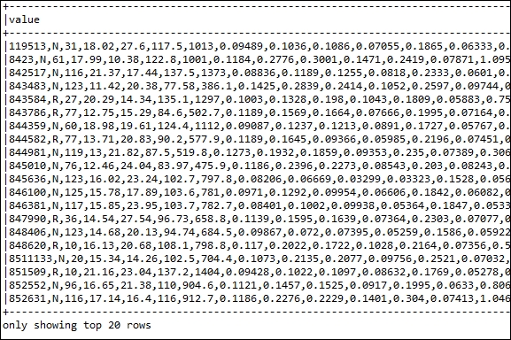
Figure 7: Sample output toward the prediction. The first value is the feature, the second is the label, and the final value is the prediction value

Now let's calculate the precision score. We do this by multiplying the counter by 100 and then dividing the value against how many predictions were done, as follows:

System.out.println("precision: " + (double) (count * 100) / predictions.count()); 
Precision - 100.0 

Therefore, the precision is 100%, which is fantastic. However, if you are still unsatisfied or have any confusion, the following chapter will demonstrate how you can still tune several parameters so that the prediction accuracy increases, as there might have been many false-negative predictions.

Furthermore, the result might vary on your platform due to the random-split nature and dataset processing on your side.