
7
The Keynesian Model of Income Determination in a Three Sector Economy: Introduction of the Government Sector
After studying this topic, you should be able to understand
- Three main activities of the government are government expenditure, transfers and taxes.
- Income leakages are in the form of saving and taxes, and injections are in the form of investment and government expenditure.
- There are two approaches to income determination in a three sector model, aggregate demand—aggregate supply approach and leakages equal injections approach.
- An economy can achieve a full employment output by an expansion in its budget, financing every rupee of additional expenditure with a rupee of additional taxes.
- Introduction of Government Transfer Payments has an expansionary effect on the income level.
- The expansionary effect on the income level will be smaller with a proportional income tax than with a lump sum income tax.
- The Government Expenditure Multiplier, Tax Multiplier and the Balanced Budget Multiplier—all have an impact on the equilibrium level of income.
INTRODUCTION
Initial chapters have focused on income determination and the multiplier in a two sector economy, where there exist the households and the firms. This chapter focuses on extending the theory of income determination and the multiplier to a three sector model, the third sector being the government sector.
The action of the government relating to its expenditures, transfers and taxes is called the fiscal policy. Here, we focus on three fiscal policy models which are in increasing order of complexity, with the emphasis being on the government expenditure, taxation and the income level. We also discuss some of the fiscal policy multipliers, including the balanced budget multiplier.
Fiscal policy relates to the actions of the government regarding its expenditures, transfers and taxes.
DETERMINATION OF EQUILIBRIUM INCOME OR OUTPUT IN A THREE SECTOR ECONOMY
Though the government is involved in a variety of activities, three of them are of greater relevance to us in the present context. Hence, we will focus on these activities of the government, which are discussed below:
- Government expenditure (or spending) includes goods purchased by the central, state and the local governments and also the payments made to the government employees.
- Transfers are those government payments which do not involve any direct services by the recipient; for example welfare payments, unemployment insurance and others.
- Taxes that include taxes on property, income and goods. Taxes can be classified into two categories, direct taxes and indirect taxes. Direct taxes are levied directly and include personal income and corporate income taxes. Indirect taxes are levied indirectly and include sales tax and excise tax. They are paid as a part of the price of the goods.
Direct taxes are levied directly and include personal income and corporate income taxes.
Indirect taxes are levied indirectly and include sales tax and excise tax. They are paid as a part of the price of the goods.
We simplify our analysis by making a few assumptions, which are as follows:
- The government purchases factor services from the household sector and goods and services from the firms.
- Transfer payments include subsidies to the firms and pensions to the household sector.
- The government levies only direct taxes on the household sector.
Transfer payments are those government payments which do not involve any direct services by the recipient, for example welfare payments, unemployment insurance and others.
We here introduce the notion of an income leakage and an injection. In a two sector model, a part of the current income stream (which was not spent on consumption) ‘leaked’ out as saving whereas injections in the form of ‘investment’ were injected into the system. In a three sector model taxes, like saving, are income leakages whereas government expenditures, like investment, are injections.
First Model of Income Determination (Introducing Government Expenditure and Tax)
This model is an extension of the two sector model with the following modifications:
- Government expenditure is determined autonomously.
- There is only one kind of tax, lump sum income tax (which is independent of the income level).
- The government expenditure equals the tax revenue. This implies that the government follows a balanced budget.
Given the above modifications, we can now analyse the equilibrium in a three sector model.
Equilibrium Income and Output
(1) Aggregate Demand–Aggregate Supply Approach
Aggregate demand = Total value of output (or income)
or
| where, | C = | Ca + bYd (consumption function) |
| Yd = | Y − T = disposable income | |
| T = | ||
| I = | ||
| G = |
Substituting for these values in the basic Eq. (1), we get
Y = Ca + bYd + ![]() +
+ ![]()
Y = Ca + b(Y − ![]() ) +
) + ![]() +
+ ![]()
Or
Y − bY = Ca + ![]() +
+ ![]() − b
− b![]()
Or
Y(1 − b) = Ca + ![]() +
+ ![]() − b
− b![]()
Thus,
Equation (2) gives the equilibrium income in a three sector economy.
(2) Leakages Equal Injections Approach
In equilibrium, in a three sector model,
AD = AS
or
C + I + G = C + S + T
As C is common in both the sides, the equilibrium condition can be written as
| where, | I = | |
| G = | ||
| S = | Yd − C = saving function | |
| C = | Ca + bYd (consumption function) | |
| T = |
Substituting for these values in the Eq. (3), we get
![]() +
+ ![]() = S +
= S + ![]()
![]() +
+ ![]() = (Yd − C) +
= (Yd − C) + ![]()
![]() +
+ ![]() = [Y −
= [Y − ![]() − (Ca + bYd)] +
− (Ca + bYd)] + ![]()
![]() +
+ ![]() = [Y −
= [Y − ![]() − Ca − b(Y −
− Ca − b(Y − ![]() )] +
)] + ![]()
Y − bY = Ca + ![]() +
+ ![]() − b
− b![]()
Y (1 − b) = Ca + ![]() +
+ ![]() − b
− b![]()
or
Y (1 − b) = Ca + ![]() +
+ ![]() − b
− b![]()
Thus,
The above equation is the same as Eq. (2) above. Hence, both the approaches yield the same equilibrium level of income.
Equilibrium Income and Output: A Graphical Explanation
(1) Aggregate Demand–Aggregate Supply Approach
Equilibrium: The determination of the equilibrium income by the aggregate demand–aggregate supply approach in a three sector economy has been depicted in the Figure 7.1 (a).
| where, | x-axis = | disposable income |
| y-axis = | aggregate demand or aggregate planned expenditure | |
| C = | aggregate consumption function, C = Ca + bYd = Ca + b(Y – |
|
| Ca = | the intercept of the consumption function on the y axis showing consumption spending at zero income level. | |
| b = | the MPC or the slope of the consumption function (it will remain constant since, in our analysis, the consumption function is a linear function.) | |
| I = | ||
| G = | ||
| AD1 = | aggregate demand function before a tax (which is obtained by adding the consumption function, the investment function and the government expenditures) | |
| AS = | aggregate supply function (also called the guideline or the 45 degree line) | |
| Point E = | the two sector equilibrium or the initial equilibrium where the aggregate demand curve AD (C + I) and aggregate supply curves intersect to determine the equilibrium income at Y*. |

Figure 7.1 Determination of Equilibrium Income or Output in a Three Sector Economy
A balanced budget exists when the entire government expenditure is financed by taxes or that G = T.
| Point E1 = | the three sector equilibrium where the aggregate demand curve AD1 (C + I + G) and aggregate supply curves intersect to determine the equilibrium income at Y1. It is important to note that at this stage, the entire government expenditure is deficit financed and that the taxes are zero. Thus, increase in government spending will lead to an increase in income where ΔY > ΔG or ΔY = mΔG. Hence, the multiplier m > 1. | |
| C′ = | the consumption function after the tax. As a tax is a withdrawal, it reduces the disposable income (Yd) thus leading to a shift of the consumption function from C to C′ and a shift of the aggregate demand curve from AD1 to AD2. | |
| AD2 = | aggregate demand function after a tax | |
| Point E2 = | the three sector equilibrium where the aggregate demand curve AD2 (C′ + I + G) and aggregate supply curves intersect to determine the equilibrium income at Y2. The entire government expenditure is financed by taxes or that G = T. In other words, it is a balanced budget. |
(2) Leakages Equals Injections Approach
Equilibrium: The determination of the equilibrium income by the leakages and injections approach in a three sector economy has been depicted in the Figure 7.1(b).
| where, x-axis = | disposable income |
| y-axis = | planned saving, planned investment, taxes and government expenditure |
| S = | planned saving |
| I = | I = investment function |
| S + |
planned saving plus taxes |
| I + |
planned investment plus government expenditure |
| E = | the two sector equilibrium or the initial equilibrium where the saving curve, S and the investment curve, |
| Point E1 = | the three sector equilibrium where the saving curve, S and the investment plus government expenditure curve, |
| S′ = | saving after the imposition of the tax |
| Point E2 = | the three sector equilibrium where the planned saving and taxes curve, S′ + |
We find that the two approaches to the determination of the equilibrium income, the aggregate demand—aggregate supply approach and the leakages equals injections approach, both yield the same result.
It is important to observe that though government expenditure has an expansionary effect, taxes have a contractionary effect on the income level. However, the contractionary effect of taxes is less than the expansionary effect of government expenditure even though ΔG = ΔT. This is because though an increase in government spending is entirely an addition to the aggregate demand, an increase in T is not entirely a decrease in the aggregate demand. Some part of the increase in T involves a reduction in the savings whereas the rest is absorbed by a reduction in consumption and, hence, in aggregate demand.
Although before the imposition of the tax the equilibrium level of income was Y1, after the tax it reduces to Y2 and not to Y* (even though G = T). Hence the imposition of a tax, given the level of government expenditure, causes a reduction in the equilibrium level of income from Y1 to Y2, though it is still larger than the initial income level Y*.
An important implication for fiscal policy is that an economy can achieve full employment output by an expansion in its budget, financing every rupee of additional expenditure with a rupee of additional taxes.
RECAP
- In a three sector model, taxes and saving are the income leakages whereas government expenditures and investment are the injections.
- The First Model of Income Determination introduces government expenditure and tax.
- The two approaches to the determination of the equilibrium income, the aggregate demand—aggregate supply approach and the leakages equal injections approach, both yield the same result.
- The imposition of a tax, given the government expenditure, reduces the equilibrium level of income.
- The contractionary effect of taxes on the income level is less than the expansionary effect of government expenditure.
The fundamental equations in an economy are given as:
| C = | 150 + 0.75(Y – T) | |
| 300 T | ||
| T = | 40 + 0.2Y | |
| 150 |
Find the equilibrium level of income.
Solution
The equilibrium condition in a three sector economy is given as Y = C + I + G.
| Thus, | Y = | 150 + 0.75[Y – (40 + 0.2Y)] + 300 + 150 |
| Y = | 150 + 0.75(Y – 40 – 0.2Y) + 300 + 150 | |
| Y = | 600 + 0.75(–40 + 0.8 Y) | |
| Y = | 600 – 30 + 0.6 Y | |
| Y – | 0.6 Y = 570 | |
| 0.4Y = | 570 | |
| Y = | ||
| Y = | 1425 |
The equilibrium level of income is 1600.
Second Model of Income Determination (Introducing Government Transfer Payments)
In the first model we had included only two activities of the government, namely, government expenditure and taxes. Here in this second model, we bring transfer payments also into the picture.
As already mentioned, transfer payments are those government payments which do not involve any quid pro quo or in other words do not involve any direct services by the recipient; for example, welfare payments. Transfer payments are, in fact, just the reverse of taxes or in other words they are negative taxes. Taxes reduce the spending capacity whereas transfer payments increase the spending capacity of the households leading to, ultimately, an increase in the equilibrium level of income.
We have our basic Eq. (1) Y = C + I + G
| where, | C = | Ca + bYd = consumption function |
| Yd = | Y – T + R = disposable income | |
| T = | ||
| I = | ||
| G = | ||
| R = |
Substituting for these values in the basic equation, we get
Y = Ca + b (Y −(![]() +
+ ![]() ) +
) + ![]() +
+ ![]()
or
Y − bY = Ca + ![]() +
+ ![]() − b
− b![]() + b
+ b![]()
or
Y (1 − b) = Ca + ![]() +
+ ![]() − b
− b![]() + b
+ b![]()
Thus,
Similar to the first model, here also a change in any of the values within brackets will lead to a change in income which will be equal to the change in that particular value times the multiplier.
It is important to observe that both the transfer payments and the government expenditure have an expansionary effect on the income level. However, the expansionary effect of an increase in the transfer payments will be less than the effect of an increase in the government expenditure even though ΔG = ΔR (as long as the marginal propensity to consume is less than 1). Thus,
This is because while the entire increase in government spending is an addition to the aggregate demand, only a part of the increase in R will be an addition to the aggregate demand (through an increase in the consumption spending). Some part of the increase in R is directed towards savings. Hence, the increase in income
- in case of an increase in government expenditure is equal to the increase in the government expenditure times the multiplier;
- in case of an increase in transfers is equal to only b (b is the marginal propensity to consume) part of the increase in the transfers times the multiplier.
It is important to note that though a change in government expenditure affects aggregate demand directly, a change in transfer payments affects aggregate demand indirectly through a change in disposable income.
RECAP
- As long as the marginal propensity to consume is less than 1, the expansionary effect of an increase in transfer payments will be less than the effect of an increase in government expenditure even when ΔG = ΔR.
- A change in government expenditure affects aggregate demand directly.
- A change in transfer payments affects aggregate demand indirectly through a change in disposable income.
Third Model of Income Determination (Including Government Expenditures, Transfer Payments and Introducing Tax as a Function of the Income Level)
In recent years, a large part of the tax receipts of the government consists of personal and corporate income taxes. Other taxes like sales tax, excise duty and service taxes also vary indirectly with the income level though less as compared to personal and corporate income taxes. Thus, we introduce tax as a linear function of income in this model.
T = ![]() + t Y +
+ t Y + ![]()
| where, | T = | the total tax |
| T = | ||
| t = | proportional income tax rate (the fraction of any income that will be taxed) | |
| |
Transfers | |
| Y = | C + I + G | |
| where, | C = | Ca + bYd = consumption function |
| Yd = | Y – T + |
|
| T = | ||
| |
transfer payments | |
| I = | ||
| G = |
Substituting for these values in the Eq. (1), we get
Y = Ca + b [Y − (![]() + tY +
+ tY + ![]() )] +
)] + ![]() +
+ ![]()
or
Y − bY = Ca + ![]() +
+ ![]() − b
− b![]() − btY + b
− btY + b![]()
or
Y − bY + btY = Ca + ![]() +
+ ![]() − b
− b![]() + b
+ b![]()
Y (1 − b + bt) = Ca + ![]() +
+ ![]() − b
− b![]() + b
+ b![]()
Thus,
In the second model where the tax receipts are independent of the income level, the multiplier is larger than the multiplier in the third model where the tax receipts are dependent on the income level.
Given an increase in government expenditure, the expansion in income will be smaller with a proportional income tax than for a lump sum income tax.
RECAP
- The multiplier in the second model, where the tax receipts are independent of the income level, is larger than the multiplier in the third model where the tax receipts are dependent on the income level.
- The increase in income will be smaller in the case of a proportional income tax than for a lump sum income tax.
Numerical Illustration 2
In the Numerical Illustration 1 suppose the government transfer payments are at Rs. 60 crores. Find the equilibrium level of income.
Solution
The equilibrium condition in the three sector economy is given as Y = Ca + b (Y – ![]() +
+ ![]() ) +
) + ![]() +
+ ![]()
| Thus, | Y = | 150 + 0.75[Y – (40 + 0.2Y) + 60] + 300 + 150 |
| Y = | 150 + 0.75(Y – 40 – 0.2Y + 60) + 300 + 150 | |
| Y = | 600 + 0.75(20 + 0.8Y) | |
| Y = | 600 + 15 + 0.6Y | |
| Y – | 0.6Y = 615 | |
| 0.40 = | 615 | |
| Y = | ||
| Y = | 1537.50 |
The equilibrium level of income is 1537.50
MULTIPLIERS IN A THREE SECTOR ECONOMY—THE FISCAL MULTIPLIERS
Through its fiscal policy, the government is in a position to influence the economic activities in an economy. To what extent its fiscal operations have an impact on the equilibrium level of income depends on the fiscal multipliers. Here, we analyse three multipliers.
Government Sector Multipliers with Lump Sum Tax
Government Expenditure Multiplier: In the First Model, we had arrived at
| where, | C = | Ca + bYd (consumption function) |
| Yd = | Y – T = disposable income | |
| T = | ||
| I = | ||
| G = |
Substituting for these values in the basic Eq. (1), we get the equilibrium level of income as
Assume that there is an increase in government expenditure by ∆G. Hence,
Subtracting Eq. (2) from Eq. (3), we get
or
| where, | ∆G = change in government expenditure |
| b = marginal propensity to consume | |
| ΔY = change in income | |
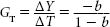
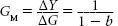
| GM = government expenditure multiplier |
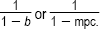
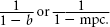
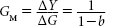
An increase in government expenditure by ΔG leads to an increase in aggregate demand and, hence, in the equilibrium level of income by ΔY. The government expenditure multiplier has the same value as the investment multiplier in the two sector model, as discussed in Chapter 5, of ![]() . As the value of b is always between 0 and 1, the multiplier will always have a value greater than 1. Hence, a change in government expenditure by ΔG will lead to a change in the equilibrium level of income by ΔY where ΔY > ΔG.
. As the value of b is always between 0 and 1, the multiplier will always have a value greater than 1. Hence, a change in government expenditure by ΔG will lead to a change in the equilibrium level of income by ΔY where ΔY > ΔG.
(1) Tax Multiplier (Lump Sum Tax)
We have Eq. (2) as
Assume that there is a change in tax by Δ![]() . Hence, we get
. Hence, we get
Subtracting Eq. (2) from Eq. (4), we get
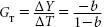
or
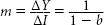
| where, | Δ |
| b = marginal propensity to consume | |
| ΔY = change in income | |
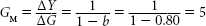
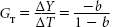
| GT = government tax multiplier |
As the tax multiplier is negative, an increase in tax leads to a decrease in the equilibrium level of income.
![]()
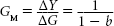
(2) The Balanced Budget Multiplier
The budget is in balance when the government expenditures plus transfer payments equal the gross tax receipts, or in other words, G = T. It follows that when there is an increase in the government expenditure, it will be financed by an increase in taxation. Thus, ΔG = ΔT.
Balanced budget multiplier is the increase in the output as a consequence of equal increases in the government expenditure and taxes.
It is important to note that an increase in the government expenditures, which is balanced by an increase in taxes of an equal amount, will not leave the income level unchanged. In fact, there will be an increase in income by the same amount as the increase in the government expenditures and the tax. This implies that it is incorrect to assert that government expenditures and taxes of an equivalent amount off set one another and that there is no increase in the income level if the budget is balanced. In fact, the increase in the income is exactly equal to the amount by which there is an increase in the government expenditures and tax. Hence the value of the ‘balanced budget’ multiplier, which is the increase in the output as a consequence of equal increases in the government expenditure and taxes, is equal to one. This is what is known as the ‘balanced budget’ or ‘unit multiplier’ theorem.
We have Eq. (2) as
Assume that there is a change in government expenditure by ΔG and in tax by ΔT, and ΔG = ΔT; hence, we get
Subtracting Eq. (2) from Eq. (5), we get
But
ΔG = ΔT
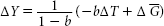
Thus, we can write
or
ΔY(1 − b) = Δ![]() (−b + 1)
(−b + 1)
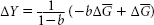
or
ΔY(1 − b) = Δ![]() (1 −b)
(1 −b)
or
| where, | ΔG = change in government expenditure |
| ΔT = change in tax | |
| b = marginal propensity to consume | |
| ΔY = change in income |
Alternatively, the balanced budget multiplier can also be obtained by summing up the government expenditure multiplier and the tax multiplier to get
The budget is in balance when the government expenditures plus transfer payments equal the gross tax receipts, or in other words, G = T.
Whatever the value of b, the sum of the government expenditure multiplier and the tax multiplier will always be equal to unity.
Regardless of the value of b (the marginal propensity to consume), the government expenditure multiplier will always be one greater than the tax multiplier.
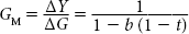
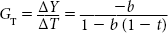
Government Sector Multipliers with Income Tax
- Government Expenditure Multiplier
- Tax Multiplier (Lump Sum Tax)
- The government expenditure multiplier has the same value as the investment multiplier, of
- As the tax multiplier is negative, an increase in tax will lead to a decrease in the equilibrium level of income.
- The value of the government expenditure multiplier will always be one greater than the value of the tax multiplier.
- An increase in the government expenditures, which is balanced by an increase in taxes of an equal amount, will lead to an increase in income by the same amount as the increase in the government expenditures and the tax.
SUMMARY
INTRODUCTION
- The present chapter focused on income determination and the multiplier to a three sector model, the third sector being the government sector.
- The action of the government relating to its expenditures, transfers and taxes is called the fiscal policy.
DETERMINATION OF EQUILIBRIUM INCOME OR OUTPUT IN A THREE SECTOR ECONOMY
- Three activities of the government are important: government expenditure, transfers and taxes.
- We simplify our analysis by making a few assumptions like the government levies only direct taxes on the household sector.
- In a three sector model, taxes are income leakages whereas government expenditures are injections.
FIRST MODEL OF INCOME DETERMINATION (INTRODUCING GOVERNMENT EXPENDITURE AND TAX)
- This model is an extension of the two sector model in that it includes autonomous government expenditure and a lump sum income tax. Also
 he government follows a balanced budget, or
  =
=  .
. - There are two approaches to the determination of equilibrium income and output: aggregate demand–aggregate supply approach and leakages equal injections approach. Both the approaches yield the same equilibrium level of income.
- The contractionary effect of taxes is less than the expansionary effect of government expenditure, even when G = T.
SECOND MODEL OF INCOME DETERMINATION (INTRODUCING GOVERNMENT TRANSFER PAYMENTS)
- In this model, in addition to the government expenditure and taxes, we bring transfer payments also into the picture.
- Transfer payments are just the reverse of taxes or, in other words, they are negative taxes.
- Taxes reduce the spending capacity whereas transfer payments increase the spending capacity of the households leading to, ultimately, an increase in the equilibrium level of income.
- The expansionary effect of an increase in transfer payments will be less than the effect of an increase in government expenditure, even when ΔG = ΔR.
- It is important to note that while a change in government expenditure affects aggregate demand directly, a change in transfer payments affects aggregate demand indirectly through a change in disposable income.
THIRD MODEL OF INCOME DETERMINATION (INCLUDING GOVERNMENT EXPENDITURES, TRANSFER PAYMENTS AND INTRODUCING TAX AS A FUNCTION OF THE INCOME LEVEL)
- In this model, tax is a linear function of income.
- In the model where the tax receipts are independent of the income level, the multiplier is larger than the multiplier in the model where the tax receipts are dependent on the income level.
- Given an increase in government expenditure, the expansion in income will be smaller with a proportional income tax than for a lump sum income tax.
MULTIPLIERS IN A THREE SECTOR ECONOMY–THE FISCAL MULTIPLIERS
- To what extent fiscal operations of the government have an impact on the equilibrium level of income depends on the fiscal multipliers.
- Government Expenditure Multiplier:
- The government expenditure multiplier has the same value as the investment multiplier of
- Tax Multiplier:
As the tax multiplier is negative, an increase in tax leads to a decrease in the equilibrium level of income.
- Whatever the value of b, the sum of the government expenditure multiplier and the tax multiplier will always be equal to unity.
- The budget is in balance when ΔG = ΔT.
- An increase in the government expenditures, which is balanced by an increase in taxes of an equal amount, will lead to an increase in income by the same amount as the increase in the government expenditures and the tax.
- The value of the ‘balanced budget’ multiplier, which is the increase in the output as a consequence of equal increases in the government expenditure and taxes, is equal to one.
- The sum of the government expenditure multiplier and the tax multiplier will always be equal to unity.
REVIEW QUESTIONS
TRUE OR FALSE QUESTIONS
- The action of the government relating to its expenditures, transfers and taxes is called the monetary policy.
- In a three sector model while taxes are income leakages, government expenditures are injections.
- The contractionary effect of taxes is less than the expansionary effect of government expenditure on the income level, even though G = T.
- Transfer payments are just the reverse of taxes or, in other words, they are negative taxes.
- The sum of the government expenditure multiplier and the tax multiplier will always be equal to unity.
VERY SHORT-ANSWER QUESTIONS
- Discuss the assumptions necessary for the determination of the equilibrium income in a three sector economy.
- What are income leakages and injections?
- Discuss the modifications in the First Model of Income Determination (including government expenditure and lump sum tax).
- ‘Whatever the value of b, the sum of the government expenditure multiplier and the tax multiplier will always be equal to unity.’ Prove.
- ‘It is incorrect to assert that government expenditures and taxes of an equivalent amount off set one another and that there is no increase in the income level if the budget is balanced’ Explain.
SHORT-ANSWER QUESTIONS
- Show as to how the imposition of a tax, given the level of government expenditure, causes a reduction in the equilibrium level of income in a three sector economy.
- The contractionary effect of taxes is less than the expansionary effect of government expenditure on the income level even though G = T. Explain.
- Differentiate between the expansionary effect of an increase in transfer payments and that of an increase in government expenditure.
- How is income determined in a model where there exists government expenditure, transfer payments and proportional income tax? Explain.
- A change in government expenditure by ΔG will lead to a change in the equilibrium level of income by ΔY where ΔY > ΔG. Explain.
LONG-ANSWER QUESTIONS
- Discuss the two approaches to the First Model of income determination (including government expenditure and tax).
- How is income determined in a model where there exists government expenditure, lump sum income taxes and transfer payments? Explain.
- Compare the model where there exists government expenditure, transfer payments and lump sum income tax with one where there exists government expenditure, transfer payments and proportional income tax.
- Write short notes on the following:
- Government expenditure multiplier
- Tax multiplier
- What is the balanced budget multiplier? Discuss.
SOLVED NUMERICAL PROBLEMS
Numerical Problem 1
In a two sector economy, the basic equations are as follows: the consumption function is C = 100 + 0.80 Yd and investment is - I = 150 crores. The equilibrium level of income is Rs. 1250 crores. Suppose the government sector is added to this two sector model, which then becomes a three sector economy. The government expenditure is at Rs. 50 crores.
- Find the equilibrium level of income in the three sector economy.
- What is the multiplier affect of the government expenditure? Is it of the same magnitude as the multiplier effect of a change in the autonomous investment?
- Suppose that there is a balanced budget in that the entire government expenditure is financed from a lump sum tax. Find the new equilibrium level of income in the three sector economy.
Numerical Problem 2
In an economy, the full employment output occurs at Rs. 1000 crores. The marginal propensity to consume is 0.80 and the equilibrium level of output is currently at Rs. 800 crores. Suppose the government aspires to achieve the full employment output, find the change in
- the level of government expenditures
- net lump sum tax
- the level of government expenditures and the net lump sum tax when the government aims at bringing the output to the full employment while keeping the budget balanced.
Numerical Problem 3
Suppose the consumption function is C = 50 + 0.80Yd and investment is ![]() = 100 crores. The government expenditure is at Rs. 90 crores whereas the tax function is a proportional income tax function where T = 0.10 Y.
= 100 crores. The government expenditure is at Rs. 90 crores whereas the tax function is a proportional income tax function where T = 0.10 Y.
- Find the equilibrium level of income in the three sector economy.
- Find the revenue from taxes at the equilibrium level of income. Is the government budget balanced?
- Suppose there is an increase in investment from Rs. 100 crores to Rs. 120 crores; what is the equilibrium level of income?
- What is the revenue from taxes at the new equilibrium level of income? Is there a balanced government budget?
Numerical Problem 4
In an economy, the marginal propensity to consume is 0.80. The tax is a lump sum tax or, in other words, not related to the income level. Find the change in the equilibrium output for the following:
- Increase in government expenditure by 10 crores.
- Increase in taxes by 15 crores.
- Increase in transfers by 10 crores.
Numerical Problem 5
In an economy, C = 50 + 0.80 Yd, ![]() = 100 crores, government expenditure is at Rs. 50 crores whereas T = 20 crores.
= 100 crores, government expenditure is at Rs. 50 crores whereas T = 20 crores.
- Find the equilibrium level of income in the three sector economy.
- Find the equilibrium level of consumption and saving at the equilibrium level of income.
- Depict the injections leakages equality at the equilibrium level.
UNSOLVED NUMERICAL PROBLEMS (WITH ANSWERS)
- Given the proportional tax function as t = 10% = 0.1 and the marginal propensity to consume as 0.75, find the change which will occur in the equilibrium level of income when there is
- an increase in government expenditure by 100.
- an increase in autonomous tax by 150.
- an increase in transfers by 150.
- In an economy, the full employment output occurs at Rs. 800 crores. The marginal propensity to consume is 0.75 and the equilibrium level of output is currently at Rs. 700 crores. Suppose the government aspires to achieve the full employment output, find the change in
- the level of government expenditures.
- net lump sum tax.
- the level of government expenditures and the net lump sum tax when the government aims at bringing the output to the full employment while keeping the budget balanced.
- In an economy, the consumption function is C = 100 + 0.75 Yd and investment is
 = 200 crores. The government expenditure is at Rs. 180 crores whereas the tax function is a proportional income tax function where T = 0.10 Y.
- Find the equilibrium level of income in the three sector economy.
- Find the revenue from taxes at the equilibrium level of income. Is the government budget balanced?
- Suppose there is an increase in investment from Rs.. 200 crores to Rs. 350 crores, what is the equilibrium level of income?
- What is the revenue from taxes at the new equilibrium level of income? Is there a balanced government budget?
- Given the marginal propensity to consume as 0.75 and the proportional tax function as t = 20% = 0.2. Find the change which will occur in the equilibrium level of income when there is
- an increase in government expenditure by 50.
- an increase in autonomous tax by 30.
- an increase in transfers by 20.
- In an economy, the consumption function is C = 40 + 0.80 Yd and investment is = 80 crores. The government expenditure is at Rs. 40 crores whereas the tax is a lump sum tax where T = 0.10.
- Find the equilibrium level of income in the three sector economy.
- Find the equilibrium level of consumption and saving at the equilibrium level of income.
- Depict the injections leakages equality at the equilibrium level.
ANSWERS
TRUE OR FALSE QUESTIONS
- False. The actions of the government relating to its expenditures, transfers and taxes is called the fiscal policy.
- True. In a three sector model, taxes and saving are income leakages whereas government expenditures and investment are injections.
- True. This is because while an increase in government spending is entirely an addition to the aggregate demand, an increase in T is not entirely a decrease in the aggregate demand. Some part of the increase in T involves a reduction in the savings whereas the rest is absorbed by a reduction in consumption and hence in aggregate demand.
- True. Taxes reduce the spending capacity whereas transfer payments increase the spending capacity of the households leading to, ultimately, an increase in the equilibrium level of income.
- False. Whatever is the value of b, the sum of the government expenditure multiplier and the tax multiplier will always be equal to unity.
SOLVED NUMERICAL PROBLEMS
Solution 1
- The equilibrium condition in the three sector economy is given as Y = C + I + G.
Thus, Y = 100 + 0.80 Y + 150 + 50 Y – 0.80Y = 100 + 150 + 50 0.20Y = 300 Y = 300/0.20 Y = 1500 The equilibrium level of income in the three sector economy is Rs. 1500 crores, which is an increase by Rs. 250 crores over the two sector economy.
- Government Expenditure Multiplier:
Investment Multiplier,
(where b is the marginal propensity to consume)
Thus, the magnitude of the multiplier effect (of a change in the autonomous investment) is the same as that of a change in government expenditure.
- G = T = Rs. 50 crores
Thus, C = 100 + 0.80(Y – 50) C = 100 – 40 + 0.80Y C = 60 + 0.80Y But Y = C + I + G Y = 60 + 0.80Y + 150 + 50 Y – 0.80Y = 60 + 150 + 50 0.20Y = 260 Y = 26/0.20 Y = 1300 The new equilibrium level of income in the three sector economy, when there exists a balanced budget, is Rs. 1300 crores.
Solution 2
- We have
where, ∆G = change in government expenditure b = marginal propensity to consume ∆Y = change in income GM = government expenditure multiplier For example,
b = 0.80
ΔY = 1000 − 800 = 200
Thus,

ΔG = 200(0.20) = 40
Thus, the level of government expenditures required to achieve the full employment output is Rs. 40 crores.
- We have
where ∆T = change in tax b = marginal propensity to consume ∆Y = change in income GT = government tax multiplier As the tax multiplier is negative, an increase in tax leads to a decrease in the equilibrium level of income.
For example,b = 0.80
ΔY = 1000 − 800 = 200
Thus,

−0.80ΔT = 200(0.20) = −50
The net lump sum tax is Rs. –50 crores. There should be a decrease in lump sum tax by Rs. 50 crores.
- Equation (8) is
But
ΔG = ΔT
Thus, we can write
or
ΔY(1 − b) = Δ ![]() (−b + 1)
(−b + 1)
or
ΔY(1 − b) = Δ G (1 − b)
or
Thus,
ΔY = ΔG = Rs. 200 crores.
The required increase in the level of government expenditures and the net lump sum tax is Rs. 200 crores.
Solution 3
- The equilibrium condition in the three sector economy is given as Y = C + I + G
Here C = 50 + 0.80Yd C = 50 + 0.80(Y − T) C = 50 + 0.80(Y − 0.10Y) C = 50 + 0.80 (0.9Y) C = 50 + 0.72Y Thus, Y = 50 + 0.72Y + 100 + 90 Y − 0.72Y = 50 +100 + 90 0.28Y = 240 Y = 240/0.28 Y = 85.71 The equilibrium level of income is Rs. 857.14 crores.
- The revenue from taxes at the equilibrium level of income.
The tax function is a proportional income tax function where T = 0.10 Y.
Thus, T = 0.10(857.14) = 85.71 crores
Hence, the revenue from taxes at the equilibrium level of income is Rs. 85.71 crores whereas the government expenditure is at Rs. 90 crores. Therefore, there is a budget deficit of Rs. 4.29 crores.
- When there is an increase in investment from Rs. 100 crores to Rs. 120 crores,
Y = 50 + 0.72Y + 120 + 90
Y − 0.72Y = 50 + 120 + 90
Y = 260/0.28
Y = 928.57
The equilibrium level of income is Rs. 928.57 crores.
- The revenue from taxes at the new equilibrium level of income is
T = 0.10(928.57) = 92.857 crores
Hence, the revenue from taxes at the equilibrium level of income is Rs. 92.857 crores whereas the government expenditure is at Rs. 90 crores. Therefore, there is a budget surplus of Rs. 2.857 crores. Due to the higher income level, there are larger tax revenues leading to a budget surplus.
Solution 4
- We have
For example, b = 0.80 and ∆G = 10.
Thus,
Thus for a 10 crore increase in the level of government expenditures, the equilibrium output increases by 50 crores.
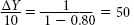
- We have
For example,
b = 0.80
∆T = 15
Thus,
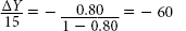
Thus, for a 15 crore increase in taxes, the equilibrium output decreases by 60 crores.
- When transfers are at 10 crores,
Thus, a 10 crore increase in transfers, increases the equilibrium output by 40 crores.
Solution 5
- The equilibrium condition in the three sector economy is given as Y = C + I + G
Here C = 50 + 0.80Yd C = 50 + 0.80(Y − T) C = 50 + 0.80(Y − 20) C = 50 + 0.80Y − 16 C = 50 + 0.80Y − 16 Thus, Y = 50 + 0.80Y − 16 + 100 + 50 Y − 0.8Y = 50 − 16 + 100 + 50 0.2Y = 184 Y = 184/0.2 Y = 920 The equilibrium level of income is Rs. 920 crores.
- When the equilibrium level of income is Rs. 920 crores,
Equilibrium level of consumption:
C = 50 + 0.80Yd C = 50 + 0.80(Y − T) C = 50 + 0.80(Y − 20) C = 50 + 0.80 Y − 16 C = 50 + 0.80Y − 16 C = 50 + 0.80 (920) − 16 C = 770 The equilibrium level of consumption is 770 crores.
Equilibrium level of saving: S = Y – C – T
S = 920 – 770 – 20 = 130
The equilibrium level of saving is 130 crores.
- Injections = I + G = 100 + 50 = 150
Leakages = S + T = 130 + 20 = 150
This depicts the injections leakages equality at the equilibrium level.
UNSOLVED NUMERICAL PROBLEMS
- (a) The equilibrium level of income increases by 307.70 when there is an increase in government expenditure by 100.
(b) The equilibrium level of income decreases by 346.15 when there is an increase in autonomous tax by 150.
(c) The equilibrium level of income decreases by 230.77 when there is an increase in transfers by 150.
- (a) The level of government expenditures required to achieve the full employment output is Rs. 25 crores.
(b) There should be a decrease in lump sum tax by Rs. 33.33 crores.
(c) The required increase in the level of government expenditures and the net lump sum tax is Rs. 100 crores.
- (a) The equilibrium level of income is Rs. 1476.92 crores.
(b) The revenue from taxes at the equilibrium level of income is Rs. 147.692 crores whereas the government expenditure is at Rs. 180 crores. Therefore, there is a budget deficit of Rs. 32.31 crores.
(c) The equilibrium level of income is Rs. 1938.46 crores.
(d) The revenue from taxes at the equilibrium level of income is Rs. 193.846 crores whereas the government expenditure is at Rs. 180 crores. Therefore, there is a budget surplus of Rs. 13.84 crores.
- (a) The equilibrium level of income increases by 125 when there is an increase in government expenditure by 50.
(b) The equilibrium level of income decreases by 56.25 when there is an increase in autonomous tax by 150.
(c) The equilibrium level of income decreases by 37.5 when there is an increase in transfers by 150.
- (a) The equilibrium level of income is Rs. 760 crores.
(b) The equilibrium level of consumption is 640 crores.
The equilibrium level of saving is 130 crores.(c) Injections = I + G = 80 + 40 = 120
Leakages = S + T = 110 + 10 = 120
This depicts the injections leakages equality at the equilibrium level.