
8
The Keynesian Model of Income Determination in a Four Sector Economy: Introduction of the Foreign Sector
After studying this topic, you should be able to understand
- In a four sector economy, the export and Import of goods and services affect the level of aggregate demand.
- There are two approaches to the determination of the equilibrium Income and output, the aggregate demand—aggregate approach and supply leakages equals injections approach.
- Transfer payments increase the equilibrium level of income.
- The four sector equilibrium exists where the C + I + G + X – M curve and aggregate supply curve intersect.
- A zero marginal propensity to import implies a multiplier, which has the same value as the ordinary multiplier.
- In an open economy, the value of the multiplier is less than that in a closed economy.
INTRODUCTION
The earlier chapters have focused on income determination in two and three sector models. Thus, the economy that was analysed was a closed economy which is in isolation from the rest of the world. This chapter presents a more realistic picture in that it focuses on a four sector model, or in other words an open economy, which is engaged in trade with the rest of the world. Thus, the aggregate demand will be now determined by the spending of four sectors, namely, households, firms, government and the foreign sector. The foreign sector will include the foreign consumers, the foreign business and the foreign governments.
The chapter also discusses the foreign trade multiplier.
DETERMINATION OF EQUILIBRIUM INCOME OR OUTPUT IN A FOUR SECTOR ECONOMY
The inclusion of the foreign sector in our analysis influences the level of aggregate demand through the export and import of goods and services. Hence, it is necessary to understand the factors that influence the exports and imports.
Open economy is an economy which is engaged in trade with the rest of the world.
The volume of exports in any economy depends on the following factors:
- The prices of the exports in the domestic economy relative to the price in the other economies.
- The income level in the other economies.
- Tastes, preferences, customs and traditions in the other economies.
- The tariff and trade policies between the domestic economy and the other economies.
- The domestic economy’s level of imports.
To simplify our analysis we assume that the exports in any economy are determined by external factors, or in other words forces which are external to the domestic economy. Thus, the level of exports is assumed to be an autonomous variable.
As far as imports are concerned, the volume of imports in any economy depends on the following factors:
- The prices of the imports relative to the domestic prices.
- The income level in the domestic economy.
- The tastes and preferences for imports as compared to the domestic goods.
- The tariff and trade policies of the domestic economy vis á vis the other economies.
- The domestic economy’s exchange rate policies.
The marginal propensity to import is the fraction of any change in income that will be devoted to imports.
To simplify our analysis, we assume that the imports in any economy are determined by the income level in the domestic economy. This brings us to the import function, which in its simplest form can be expressed as a linear function.
M = Ma + mY
Figure 8.1 depicts the import function as an upward sloping line and the exports function as a line parallel to the x-axis (as they are assumed to be determined autonomously).
| where, | x-axis = | income or output |
| y-axis = | level of exports and imports | |
| M = | imports | |
| Ma = | autonomous imports (imports at a theoretically zero level of income) | |
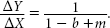
| m = | ΔM/ΔY = marginal propensity to import (fraction of any change in income that will be devoted to imports) | |
| Y = | income level |
In Figure 8.1,
- At all the income levels below Y1, as exports are greater than imports, there exists a net export balance or a favourable balance of trade.
- At all the income levels above Y1, as exports are less than imports, there exists a net import balance or an unfavourable balance of trade.
It is important to note that:
- A change in the factors that influence the exports such that there is an upward shift in the exports function will lead to an increase in the net export balance or a decrease in the net import balance at each income level.
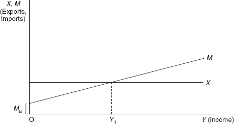
Figure 8.1 The Import and Export Functions
- A change in the factors that influence the imports such that there is a downward shift in the imports function (a decrease in Ma) or a decrease in the slope of the import function (decrease in m) will lead to an increase in the net export balance or a decrease in the net import balance at each income level.
Exports, imports and aggregate demand: While exports must be added to the total final expenditures to arrive at the aggregate demand, all the spending on imports do not contribute to the domestic demand, and thus must be deducted from the total final expenditures to arrive at the aggregate demand.
RECAP
- The level of exports is assumed to be an autonomous variable.
- The imports in any economy are determined by the income level in the domestic economy.
- When exports are greater than imports, there exists a net export balance or a favourable balance of trade.
- While exports need to be added to the total final expenditures, imports need to be deducted from the total final expenditures to arrive at the aggregate demand.
EQUILIBRIUM INCOME AND OUTPUT
- Aggregate Demand–Aggregate Supply Approach
Aggregate demand = Total value of output (or income)
or

where C = Ca + b Yd = consumption function Yd = Y – T = disposable income T =  = tax (lump sum income tax)
I = I = investment (assumed to be autonomous) G =  goverment expenditure (assumed to be autonomous)
X =  = exports (assumed to be autonomous)
M = Ma + mY =imports function Substituting for these values in the basic Eq. (1), we get
Y = Ca + bYd +
 +
+  +
+  – (Ma + mY)
Y = Ca + b(Y – T) +
+ + – Ma – mYor
Y – bY + mY = Ca +
+ + – b – Ma
– Maor
Y (1 – b + m) = Ca +
+ + – b – MaThus,

- Leakages Equal Injections Approach
In equilibrium in a four sector model,AD = AS
or
C + I + G + X = C + S + T + M
(In a four sector model, the injections include investment, government expenditures and exports whereas the leakages include saving, taxes and imports.)
As C is common in both the sides, the equilibrium condition can be written as
| where, | I = |
| G = |
|
| X = |
|
| S = Yd – C = saving function | |
| C = Ca + b Yd (consumption function) | |
| T = |
|
| M = Ma + mY (imports function) |
Substituting for these values in the Eq. (3), we get
![]() +
+ ![]() +
+ ![]() = S +
= S + ![]() + Ma + mY
+ Ma + mY
![]() +
+ ![]() +
+ ![]() = (Yd – C) +
= (Yd – C) + ![]() + Ma + mY
+ Ma + mY
![]() +
+ ![]() +
+ ![]() = {Y –
= {Y – ![]() – [Ca + b Yd} +
– [Ca + b Yd} + ![]() + Ma + mY
+ Ma + mY
![]() +
+ ![]() +
+ ![]() = {Y –
= {Y – ![]() – Ca – b(Y –
– Ca – b(Y – ![]() )} +
)} + ![]() + Ma + mY
+ Ma + mY
Y – bY + mY = Ca + ![]() +
+ ![]() +
+ ![]() – b
– b ![]() + Ma
+ Ma
Y (1 – b + m) = Ca + ![]() +
+ ![]() +
+ ![]() – b
– b ![]() – Ma
– Ma
Thus,
![]() (Ca +
(Ca + ![]() +
+ ![]() +
+ ![]() – b
– b ![]() – Ma)
– Ma)
The above equation is the same as Eq. (2) above. Hence, both the approaches yield the same equilibrium level of income.
RECAP
- Both the approaches to income determination yield the same equilibrium level of income.
INTRODUCTION OF GOVERNMENT TRANSFER PAYMENTS IN A FOUR SECTOR MODEL
Till now, we have not included transfer payments in our analysis. As already mentioned transfer payments increase the spending capacity of the households, leading to an increase in the equilibrium level of income.
We have our basic Eq. (1)
| Y = C + I + G + X – M | |
| where, | C = Ca + bYd = consumption function |
| Yd = Y – T + R = disposable income | |
| T = |
|
| I = |
|
| G = |
|
| X = |
|
| M = Ma + mY = imports | |
| R = |
Substituting for these values in the basic equation, we get
Y = Ca + b (Y – ![]() +
+ ![]() ) +
) + ![]() +
+ ![]() +
+ ![]() – Ma – mY
– Ma – mY
or
Y – bY + mY = Ca + ![]() +
+ ![]() +
+ ![]() – b
– b![]() + bR + Ma
+ bR + Ma
or
Y (1– b + m) = Ca + ![]() +
+ ![]() +
+ ![]() – b
– b ![]() + bR + Ma
+ bR + Ma
Thus,
Determination of Equilibrium Income and Output: A Graphical Explanation
Aggregate Demand–Aggregate Supply Approach
Equilibrium: The determination of the equilibrium income by the aggregate demand–aggregate supply approach in a four sector economy has been depicted in the Figure 8. 2(a).
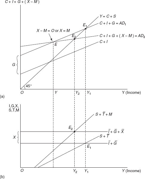
Figure 8.2 Determination of Equilibrium Income or Output in a Four Sector Economy
At point E, curves AD1 and AD2 intersect to determine the equilibrium income at Y. At this level of income, exports equal imports or X = M.
To the left of point E, curve AD2 is above AD1 indicating that exports exceed imports or X > M.
To the right of point E, curve AD2 is below AD1 indicating that imports exceed exports or X < M.
Leakages Equals Injections Approach
Equilibrium: The determination of the equilibrium income by the leakages and injections approach in a four sector economy has been depicted in the Figure 8.2(b).
The leakages now include saving, taxation and imports whereas the injections are investment, government expenditure and imports.
| where, | x-axis | = disposable income |
| y-axis | = planned saving, planned investment, taxes and government expenditure, exports and imports | |
| S | = planned saving | |
| I | = |
|
| X | = |
|
| M | = imports function | |
| S + |
= planned saving plus taxes plus imports | |
| = planned investment plus government expenditure plus exports | ||
| Point E1 | = the three sector equilibrium where the planned saving and taxes curve, S + |
|
| Point E2 | = the four sector equilibrium where the planned saving, taxes and imports curve, S + |
We find that in a four sector economy the two approaches to the determination of the equilibrium income, the aggregate demand-aggregate supply approach and the leakages equal injections approach, both yield the same result.
The introduction of foreign trade has the affect of reducing the equilibrium level of income from Y1 to Y2.
RECAP
- In an economy, the exports are assumed to be exogenous whereas the imports are assumed to be a linear function of the income level.
- At the level of income where the C + I + G and C + I + G + X – M curves intersect, exports equal imports or X = M.
- The introduction of foreign trade has the affect of reducing the equilibrium level of income.
MULTIPLIER IN A FOUR SECTOR ECONOMY—THE FOREIGN TRADE MULTIPLIER
To have an understanding of the multiplier in the foreign sector, we assume that due to an increase in the income level in the other countries there occurs an increase in the exports of the domestic country. To meet this increased demand for exports, there is an increase in the domestic production which leads to an increase in the income and hence in the consumption expenditure (depending on the marginal propensity to consume). A part of this increase in the consumption expenditure will be directed towards imports, depending on the marginal propensity to import. This will further lead to a second stage of expansion; though due to the leakage from the economy in the form of imports, there will occur only a restricted increase in the income. Further increases in the income will become smaller and smaller. The size of the multiplier will be lower when the marginal propensity to import is positive.
In a four sector economy, the equilibrium level of income is
Assume that there is an increase in exports by ΔX. Hence,
Subtracting Eq. (2) from Eq. (5), we get
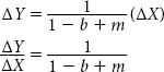
| where, | ΔX = | change in exports |
| b = | marginal propensity to consume | |
| ΔY = | change in income | |
The value of the multiplier in an open economy is less than that in a closed economy. This is because in the open economy, there is an additional leakage in the form of imports. Thus as long as the marginal propensity to import is positive, the size of the multiplier gets reduced. A zero marginal propensity to import implies a multiplier, which is the same as the ordinary multiplier, 1/1 – b.
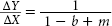
Another way of analysing the effect of the marginal propensity to import on the multiplier is by expressing the multiplier as 1/1 –(b – m).
Here, we can write
| b = | marginal propensity to purchase both domestically and foreign produced goods |
| m = | marginal propensity to purchase foreign produced goods |
| b – m = | marginal propensity to purchase domestically produced goods |
It is to be observed that
- If b = m, the value of the multiplier is equal to 1.
- If b < m, the value of the multiplier would be greater than 1.
- If the value of m were zero, then the multiplier would become equal to the ordinary multiplier.
RECAP
- When the marginal propensity to import is positive, the size of the multiplier will be lower.
- When the marginal propensity to import is zero, then the multiplier would become equal to the ordinary multiplier.
SUMMARY
INTRODUCTION
- The chapter focused on a four sector model or, in other words, an open economy which is engaged in trade with the rest of the world.
- The aggregate demand will be determined by the spending of four sectors, namely, households, firms, government and the foreign sector.
DETERMINATION OF EQUILIBRIUM INCOME OR OUTPUT IN A FOUR SECTOR ECONOMY
- The inclusion of the foreign sector influences the level of aggregate demand through the export and import of goods and services.
- The volume of exports in any economy depends on many factors including prices of the exports and income level in the other economies.
- The level of exports is assumed to be an autonomous variable.
- The volume of imports in any economy depends on many factors including the prices of the imports and the income level in the domestic economy.
- We assume that the imports in any economy are determined by the income level in the domestic economy with the import function as M – Ma + mY.
- When exports are greater than imports, there exists a net export balance or a favourable balance of trade. When exports are less than imports, there exists a net import balance or an unfavourable balance of trade.
- Although exports must be added to the total final expenditures to arrive at the aggregate demand, all spending on imports does not contribute to the domestic demand and thus must be deducted from the total final expenditures to arrive at the aggregate demand.
EQUILIBRIUM INCOME AND OUTPUT
- There are two approaches to the determination of the equilibrium income and output, the aggregate demand–aggregate supply approach where Y = C + I + G + X – M and leakages equals injections approach where I + G + X = S + T + M.
- Both the approaches yield the same equilibrium level of income.

INTRODUCTION OF GOVERNMENT TRANSFER PAYMENTS IN A FOUR SECTOR MODEL
- Transfer payments increase the spending capacity of the households leading to an increase in the equilibrium level of income.
- The equilibrium level of income is thus

EQUILIBRIUM INCOME AND OUTPUT: A GRAPHICAL EXPLANATION
- According to the aggregate demand–aggregate supply approach, in the Figure 8.2(a) the four sector equilibrium exists at point E2 where the aggregate demand curve AD2 (= C + I + G + X – M) and aggregate supply curves intersect to determine the equilibrium income at Y2.
- At point E, the curves AD1 and AD2 intersect to determine the equilibrium income at Y. At this level of income, exports equal imports or X = M.
- According the leakages equals injections approach, in the Figure 8.2(b) the four sector equilibrium exists at point E2 where the S + + M curve and + + curve intersect to determine the equilibrium income at Y2.
- The introduction of foreign trade has the affect of reducing the equilibrium level of income.
MULTIPLIER IN A FOUR SECTOR ECONOMY – THE FOREIGN TRADE MULTIPLIER
- The size of the multiplier will be lower when the marginal propensity to import is positive.
- The foreign trade multiplier can be expressed as
- The value of the multiplier in an open economy is less than that in a closed economy.
- A zero marginal propensity to import implies a multiplier which is the same as the ordinary multiplier, 1/1 – b.
- It is to be observed that if b = m, the value of the multiplier is equal to 1; if b < m, the value of the multiplier would be greater than 1; if the value of m were zero, then the value of the multiplier would become equal to the ordinary multiplier.
REVIEW QUESTIONS
TRUE OR FALSE QUESTIONS
- The level of imports is assumed to be an autonomous variable.
- The imports in any economy are determined by the income level in the domestic economy.
- When exports are greater than imports, there exists a net import balance or an unfavourable balance of trade.
- While exports must be added to the total final expenditures, imports must be deducted from the total final expenditures to arrive at the aggregate demand.
- The introduction of foreign trade has the aff ect of increasing the equilibrium level of income
VERY SHORT-ANSWER QUESTIONS
- Discuss the factors that influence the volume of exports in an economy.
- Discuss the factors that influence the volume of imports in an economy.
- Which are the two approaches to the determination of the equilibrium income and output?
- Show, diagrammatically, the significance of the point at which the level of exports equal the level of imports.
- ‘The value of the multiplier in an open economy is less than that in a closed economy.’ Explain.
SHORT-ANSWER QUESTIONS
- Describe the imports function and the exports function.
- What is the impact on the export or import balance of
- an upward shift in the exports function?
- a downward shift in the imports function?
- How does the introduction of government transfer payments affect a four sector model.
- ‘The size of the multiplier will be lower when the marginal propensity to import is positive’. Explain.
- In the foreign trade multiplier
What is the relationship between b and m? Discuss.
LONG-ANSWER QUESTIONS
- What are the assumptions necessary for the determination of equilibrium income or output in a four sector economy? Discuss.
- How is the equilibrium level of income and output determined in a four sector model? Explain using both the aggregate demand–aggregate supply and leakages equals injections approach.
- Show a graphical explanation to the determination of the equilibrium income and output in a four sector model.
- Write a short note on the foreign trade multiplier.
- Compare the equilibrium income

With

What is the difference between the two equations? Comment.
SOLVED NUMERICAL PROBLEMS
Numerical Problem 1
The fundamental equations in an economy are given as:
| Consumption function C = | 100 + 0.80 Y |
| Investment function |
150 |
| Tax T = | 60 |
| Government expenditure G = | 100 |
| Exports X = | 50 |
| Imports M = | 0.05 Y. |
Find the following:
- the equilibrium level of income.
- the net exports.
Numerical Problem 2
For the credentials of the Numerical Problem 1, find
- the increase in the income if both government expenditure and tax increased by an amount of 10 each.
- the net exports, if exports increased by an amount of 30.
- the increase in the government expenditure if the economy were to achieve the full employment income level of 1600.
Numerical Problem 3
In an economy, the following information is given:
- The level of consumption is 50 crores plus 50 per cent of each increment of the disposable income.
- Investment is fixed at 200 crores.
- Tax is fixed at 120 crores.
- Government expenditure is also fixed at 150 crores.
- Exports are at 70 crores whereas imports are at 50 crores.
Find the equilibrium level of the national income.
Numerical Problem 4
Suppose the basic functions in an economy are as follows:
| C = 130 + 0.80Yd | |
| T = 150 | |
| G = 150 | |
| X = 150 – 0.05Y |
- Find the equilibrium level of income.
- Find the net exports at equilibrium level of income.
- Find the equilibrium level of income and the net exports when there is an increase in investment from 160 to 170.
- Find the equilibrium level of income and the net exports when the net export function becomes 140 – 0.05 Y.
Numerical Problem 5
The equations in an economy are given as:
Consumption function C = 200 + bYd
Investment function ![]() = 70
= 70
Tax T = 60
Government expenditure G = 70
Exports X = 20
Imports M = 10 + 0.1 Y
Marginal propensity to consume, b = 0.8.
Find
- the equilibrium level of income.
- the value of the foreign trade multiplier.
- the equilibrium level of imports.
UNSOLVED NUMERICAL PROBLEMS (WITH ANSWERS)
- The fundamental equations in an economy are given as follows:
Consumption function C = 50 + 0.50 Yd Investment function  =
=350 Tax T = 60 Government expenditure G = 200 Exports X = 90 Imports M = 0.05Y Find
- the equilibrium level of income.
- the net exports.
- In Numerical Problem 1, find
- The fundamental equations in an economy are given as:
Consumption function C = 100 + 0.60 Yd Investment function =400 Tax T = 200 Government expenditure G = 300 Exports X = 300 Imports M = 200. Find
- the equilibrium level of income.
- the net exports.
- The following information is given in an economy:
- The level of consumption is 100 crores plus 60 per cent of each increment of the disposable income.
- Investment is fixed at 400 crores.
- Tax is fixed at 200 crores.
- Government expenditure is also fixed at 300 crores.
- Exports are at 300 crores whereas imports are at 200 crores.
Find the equilibrium level of the national income.
- Suppose the basic functions in an economy are as follows:
C = 50 + 0.60 Yd
= 60T = 30
G = 28
X = 20 + 0.05Y
- Find the equilibrium level of income.
- Find the net exports at equilibrium level of income.
- Find the equilibrium level of income and the net exports when there is an increase in investment from 60 to 95.
- Find the equilibrium level of income and the net exports when the net export function becomes 6 + 0.05 Y.
- The equations in an economy are given as:
Consumption function C = 50 + bYd Investment function =40 Tax T = 20 Government expenditure G = 40 Exports X = 20 Imports M = 20 + 0.1 Y Marginal propensity to consume, b = 0.75. Find the following:
- the equilibrium level of income.
- the value of the foreign trade multiplier.
- the equilibrium level of imports.
TRUE OR FALSE QUESTIONS
- False. The level of exports is assumed to be an autonomous variable.
- True. The import function in its simplest form can be expressed as a linear function M = Ma + mY.
- False. When exports are greater than imports, there exists a net export balance or a favourable balance of trade. When exports are less than imports, there exists a net import balance or an unfavourable balance of trade.
- True While exports must be added to the total final expenditures to arrive at the aggregate demand, all spending on imports does not contribute to the domestic demand, and thus must be deducted from the total final expenditures to arrive at the aggregate demand.
- False. The introduction of foreign trade has the aff ect of reducing the equilibrium level of income.
SOLVED NUMERICAL PROBLEMS
Solution 1
- The consumption function is
C = 100 + 0.8Yd
C = 100 + 0.8 (Y – T)
C = 100 + 0.8 (Y – 60)
The equilibrium condition is given as Y = C + I + G + X – M
Thus,
Y = 100 + 0.8 (Y – 60) + 150 + 100 + (50 – 0.05Y)
Y = 100 + 0.8 Y – 48 + 300 – 0.05Y
Y – 0.8Y + 0.05Y = 352
0.25Y = 352

Y = 1408
The equilibrium level of income is 1408.
Checking the answer
In equilibrium in a four sector model, leakages equal injections or C + I + G + X = C + S + T + M.
The consumption function is
C = 100 + 0.8 Yd
C = 100 + 0.8 (1408 – 60)
C = 100 + 0.8 (1348)
C = 1178.4
The saving function is
S = Yd – C
S = (Y – 60) – 1178.4
S = (1408 – 60) – 1178.4 = 169.6
S = 169.6
Thus,
I + G + X = S + T + M
150 + 100 + 50 = 169.6 + 60 + 0.05Y
300 = 229.6 + 0.05 (1408)
300 = 300
- Imports M = 0.05Y = 0.05 (1408) = 70.4
Net Exports: X – M = 50 – 70.4 = – 20.4
X – M = – 20.4
There is a deficit in the balance of trade.
Solution 2
- If both government expenditure and tax increased by an amount of 10 each, G = 110 and T = 70.
The equilibrium condition is given as Y = C + I + G + X – M
Thus,
Y = 100 + 0.8 (Y – 70) + 150 + 110 + (50 – 0.05Y)
Y = 100 + 0.8 Y – 56+ 310 – 0.05Y
Y – 0.8Y + 0.05Y = 354
0.25Y = 354

Y = 1416
The equilibrium level of income is 1416. Hence, there is an increase in the income level by 8.
- If exports increased by an amount of 30, X = 80.
The equilibrium condition is given as Y = C + I + G + X – M.
Thus,
Y = 100 + 0.8 (Y – 60) + 150 + 100 + (80 – 0.05Y)
Y = 100 + 0.8 Y – 48 + 330 – 0.05Y
Y – 0.8Y + 0.05Y = 382
0.25Y = 382

Y = 1528
The equilibrium level of income is 1528.
Imports M = 0.05 Y = 0.05 (1528) = 76.4
Net Exports: X – M = 80 – 76.4 = 3.6
X – M = 3.6
There is a surplus in the balance of trade.
- We have
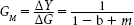
Where, ΔG =change in government expenditure b = marginal propensity to consume ΔY = change in income GM = government expenditure multiplier m = marginal propensity to import In the present example,
b = 0.80
ΔY = 1600 – 1408 = 192
Thus,
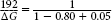
ΔG = 192 (0.25) = 48
ΔG = 48
The level of government expenditures required to achieve the full employment output is 48.
Here, we have the consumptisubon function as
C = 50 + 0.5 Yd
C = 50 + 0.5 (Y – T)
C = 50 + 0.5 (Y – 120)
The equilibrium condition is given as Y = C + I + G + X – M
Thus,
Y = 50 + 0.5 (Y – 120) + 200 + 150 + (70 – 50)
Y = 50 + 0.5 Y – 60 + 350 + 20
Y – 0.5Y = 360
0.5Y = 360
Y = 720
The equilibrium level of income is 720.
Checking the answer
In equilibrium in a four sector model, leakages equal injections
or
C + I + G + X = C + S + T + M
The consumption function is C = 50 + 0.5 Yd
C = 50 + 0.5 (720 – 120)
C = 50 + 0.5 (600)
C = 350
The saving function is S = Yd – C
S = (Y – T) – C
S = (720 – 120) – 350 = 250
S = 250
Thus,
I + G + X = C + S + T + M
200 + 150 + 70 = 250 + 120 + 50
420 = 420
Solution 4
- The consumption function is
C = 130 + 0.8Yd
C = 130 + 0.8 (Y – T)
C = 130 + 0.8 (Y – 150)
The equilibrium condition is given as Y = C + I + G + X – M.
Thus,
Y = 130 + 0.8 (Y – 150) + 160 + 150 + (150 – 0.05Y)
Y = 130 + 0.8 Y – 120 + 460 – 0.05Y
Y – 0.8Y + 0.05Y = 470
0.25Y = 470

Y = 1880
The equilibrium level of income is 1880.
- Imports M = 0
Net Exports: X – M = 150 – 0.05 (1880) – 0
X – M = 56
There is a surplus in the balance of trade.
- Y = 130 + 0.8 (Y – 150) + 170 + 150 + (150 – 0.05Y)
Y = 130 + 0.8 Y – 120 + 470 – 0.05Y
Y – 0.8 Y + 0.05Y = 480
0.25Y = 480

Y = 1920
The equilibrium level of income is 1920 which is an increase by 40.
Imports M = 0
Net Exports: X – M = 150 – 0.05 (1920)– 0
X – M = 54
- There is a surplus in the balance of trade.
Y = 130 + 0.8 (Y – 150) + 160 + 150 + (140 – 0.05Y)
Y = 130 + 0.8 Y – 120 + 450 – 0.05Y
Y – 0.8Y + 0.05Y = 460
0.25Y = 460

Y = 1840
The equilibrium level of income is 1840, which is a decrease by 40.
Imports M = 0
Net Exports: X – M = 140 – 0.05 (1840)– 0
X – M = 48
There is a surplus in the balance of trade.
Solution 5
- The consumption function is
C = 200 + 0.8Yd
C = 200 + 0.8 (Y – T)
C = 200 + 0.8 (Y – 60)
The equilibrium condition is given as Y = C + I + G + X – M
Thus,
Y = 200 + 0.8 (Y – 60) + 70 + 70 + 20 – 10 – 0.1Y
Y = 200 + 0.8Y – 48 + 150 – 0.1Y
Y – 0.6Y – 0.1Y = 302
0.3Y = 302

Y = 1006.67
The equilibrium level of income is 1006.67.
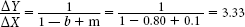
- Foreign trade multiplier
- Imports at the equilibrium level: M = 10 + 0.1Y = 10 + 0.1 (1006.67)
M = 110.67
The equilibrium level of imports is 110.67.
UNSOLVED NUMERICAL PROBLEMS
- (a) Y = 1200
The equilibrium level of income is 1200.
(b) X – M = 30
There is a surplus in the balance of trade. - (a) Y = 1400
The equilibrium level of income is 1400.
(b) Y = 1240
The equilibrium level of income is 1240.
X – M = 50
There is a surplus in the balance of trade.
(c) ΔG = 165
The level of government expenditures required to achieve the full employment output is 165.
- (a) Y = 1950
The equilibrium level of income is 1950.
(b) X – M = 100
There is a surplus in the balance of trade.
- Y = 1950
The equilibrium level of income is 1950.
- (a) Y = 400
The equilibrium level of income is 400.
(b) X – M = 40
There is a surplus in the balance of trade.
(c) Y = 500
The equilibrium level of income is 500, which is an increase by 100.
X – M = 45
There is a surplus in the balance of trade.
(d) Y = 360
The equilibrium level of income is 360.
X – M = 24
There is a surplus in the balance of trade.
- (a) Y = 328.57
The equilibrium level of income is 328.57.
(b) Foreign trade multiplier = 2.86
(c) M = 52.86
The equilibrium level of imports is 52.86.