
Chapter 12
Introducing nParticles
This chapter introduces nParticle dynamics in the Autodesk® Maya® program and shows you how you can use them creatively to produce a wide variety of visual effects. The example scenes demonstrate the fundamentals of working with and rendering particles. The subsequent chapters on Maya dynamics build on these techniques.
nParticles are connected to the Nucleus solver system, a difference from traditional Maya particles. Nucleus is a unified dynamic system that is part of nCloth. The Nucleus solver is the brain behind the nDynamic systems in Maya.
In this chapter, you will learn to
- Create nParticles
- Make nParticles collide
- Create liquid simulations
- Emit nParticles from a texture
- Move nParticles with Nucleus wind
- Use force fields
Creating nParticles
A particle is a point in space that can react to the simulated dynamic forces generated by Maya. These dynamic forces allow you to create animated effects in a way that would be difficult or impossible to create with standard keyframe animation. When you create a particle object, points are created in the scene. You can then attach force fields to the particles to push them around and make them fall, swarm, float, or perform any number of other behaviors without the need for keyframes.
Maya particle dynamics have been part of Maya since the earliest versions of the software. In Maya 2009, Autodesk introduced nParticles, which have all of the capabilities of the older, traditional particles plus additional attributes that make them easier to use and more powerful. Unlike traditional particles, nParticles can collide and influence the behavior of other nParticles. nParticle collisions occur when two or more nParticles come within a specified distance, causing them to bounce off one another or, in some cases, stick together. Very complex behaviors can be created by adjusting the settings in the nParticle’s Attribute Editor. In this chapter, you’ll learn how you can create effects by adjusting these settings. Since nParticles can do just about everything traditional particles can do and then some, traditional particles are now considered legacy features and have been moved to the nParticles menu under the Legacy Particles subheading.
An nCloth object is a piece of polygon geometry that can also react to dynamic forces. Each vertex in an nCloth object has the properties of an nParticle, and these nParticles are connected by invisible virtual springs, which means nCloth objects can collide with, and influence the behavior of, other nCloth objects and nParticles. In this chapter, you’ll get a taste of working with nCloth; Chapter 13, “Dynamic Effects,” demonstrates more advanced nCloth and nParticle effects.
When you create an nParticle object or an nCloth object (or both) in a scene, a Nucleus solver is created. The Nucleus solver is a node in Maya that acts as an engine for all of the dynamic effects. The Nucleus solver determines global settings for the dynamics, such as the strength and direction of gravity, the air density, the wind direction, and the quality of the dynamics simulation (for example, how many times per frame the simulation is calculated). The same Nucleus solver is used to calculate the dynamics and interactions within the nParticle system and the nCloth system. A scene can have more than one Nucleus solver, but nDynamic systems using two different solvers can’t directly interact. However, two separate nParticle objects using the same Nucleus solver can interact.
Traditional Maya dynamics use a much simpler solver node that does not take into account interactions between different dynamic objects. Traditional particle objects are completely self-contained, so two particle objects in a Maya scene are not aware of each other’s existence (so to speak).
The following exercises take you through the process of using the different nParticle-creation methods and introduce you to working with the Nucleus solver.
Drawing nParticles Using the nParticle Tool
You can create nParticles in a scene in a number of ways. You can draw them on the grid, use an emitter to spawn them into a scene, use a surface as an emitter, or fill a volume with nParticles. When you create an nParticle object, you also need to specify the nParticle’s style.
Choosing a style activates one of a number of presets for the nParticle’s attributes, all of which can be altered after you add the nParticle object to the scene. The nParticle styles include Balls, Point, Cloud, Thick Cloud, and Water.
The simplest way to create nParticles is to draw them on the grid using the nParticle tool, as follows:
- Create a new scene in Maya. Switch to the FX menu set.
- Choose nParticles ➢ Create Options, and set the style to Balls (see Figure 12.1).
- Choose nParticles ➢ nParticle Tool. Click six or seven times on the grid to place individual particles.
-
Press the Enter key to create the particle group.
You’ll see several circles on the grid. The ball-type nParticle style automatically creates blobby surface particles. Blobby surfaces are spheres rendered using the Maya Software or mental ray® program. Blobby surfaces use standard Maya shaders when rendered, and they can be blended together to form a gooey surface.
- Set the length of the timeline to 600. Rewind and play the animation. The particles will fall in space.
- Open the Attribute Editor for the nParticle1 object, and switch to the nucleus1 tab. The settings on this tab control the Nucleus solver, which sets the overall dynamic attributes of the connected nDynamic systems (see Figure 12.2).
- By default, a Nucleus solver has Gravity enabled. Select Use Plane in the Ground Plane settings (see Figure 12.3). This creates an invisible floor on which the nParticles can rest. Set the Plane Origin’s Translate Y to −1.
- The Nucleus solver also has wind settings. Set Wind Speed to 3 and Wind Noise to 4. By default, Wind Direction is set to 1, 0, 0 (see Figure 12.4). The fields correspond to the x-, y-, and z-axes, so this means that the nParticles will be blown along the positive x-axis. Rewind and play the animation. Now the nParticles are moving along with the wind, and a small amount of turbulence is applied.

Figure 12.1 Using the nParticle menu to specify the nParticle style

Figure 12.2 The settings on the nucleus1 tab define the behavior of the environment for all connected nDynamic nodes.

Figure 12.3 The Use Plane parameter creates an invisible floor that keeps the nParticles from falling.

Figure 12.4 You can find the settings for Air Density, Wind Speed, Wind Direction, and Wind Noise under the Nucleus solver’s attributes.
By increasing the Air Density value, you adjust the atmosphere of the environment. A very high setting is a good way to simulate an underwater environment. Using wind in combination with a high air density pushes the nParticles with more force; this makes sense because the air is denser.
The Solver Attributes section of the nParticle menu sets the quality of the solver. The Substeps setting specifies how many times per frame the solver calculates nDynamics. Higher settings are more accurate but can slow down performance. Increasing the Substeps value may alter some of the ways in which nDynamics behave, such as how they collide with each other and with other objects. Thus, when you increase this value, be aware that you may need to adjust other settings on your nDynamic nodes.
The Time Attributes section allows you to set the start time for the solver. This is useful if you have an nCloth object that does not need to do anything until a certain frame within your animation. Inversely, you can start the simulation prior to the beginning of your animation to give your nCloth object time to simulate to the desired position. Frame Jump Limit is good for previewing your simulations. Instead of having to simulate each frame, with a Frame Jump Limit value of 1.0, you can increase the limit, enabling the solver to skip over frames without error. Having a value greater than 1 will not produce an accurate simulation but will give you an idea of the final solution.
The Scale Attributes section has Time Scale and Space Scale sliders. Use Time Scale to speed up or slow down the solver. Values less than 1 slow down the simulation; higher values speed it up. If you increase Time Scale, you should increase the number of substeps in the Solver Attributes section to ensure that the simulation is still accurate. One creative example of Time Scale would be to keyframe a change in its value to simulate the “bullet time” effect made famous in The Matrix movies.
Space Scale scales the environment of the simulation. By default, nDynamics are calculated in meters even if the Maya scene unit is set to centimeters. You should set this to 0.1 if you need your nDynamics simulation to behave appropriately when the Maya scene units are set to centimeters. This is more noticeable when working with large simulations. You can also use this setting creatively to exaggerate effects or when using more than one Nucleus solver in a scene. Most of the time, it’s safe to leave this at the default setting of 1. For the following examples, leave Space Scale set to 1.
Spawning nParticles from an Emitter
An emitter shoots nParticles into the scene, like a sprinkler shooting water onto a lawn. When a particle is emitted into a scene, it is “born” at that moment, and all calculations based on its age begin from the moment it is born.
- Continue with the scene from the previous section. Add an emitter to the scene by choosing nParticles ➢ Create Emitter. An emitter appears at the center of the grid.
- Open the Attribute Editor for the emitter1 object, and set Rate (Particles/Sec) to 10. Set Emitter Type to Omni.
-
Rewind and play the scene. The Omni emitter spawns particles from a point at the center of the grid. Note that after the particles are born, they collide with the ground plane and are pushed by the Nucleus wind in the same direction as the other particles (see Figure 12.5).
The new nParticles are connected to the same Nucleus solver. If you open the Attribute Editor for the nParticle2 object, you’ll see the tabs for nucleus1 and nParticle2, as well as the tab for nParticle1. If you change the settings on the nucleus1 tab, both nParticle1 and nParticle2 are affected.
- Select nParticle2, and choose Fields/Solvers ➢ Assign Solver ➢ New Solver. Rewind and play the scene. nParticle2 now falls in space, whereas nParticle1 continues to slide on the ground plane.
- In the Outliner, you’ll see nucleus1 and nucleus2 nodes (see Figure 12.6).
- Select nParticle2, and choose Fields/Solvers ➢ Assign Solver ➢ nucleus1. This reconnects nParticle2 with nucleus1.
- Select emitter1, and in the Attribute Editor for emitter1, set Emitter Type to Volume.
- Set Volume Shape in the Volume Emitter Attributes section to Sphere.
-
Use the Move tool to position the emitter above the ground plane. The emitter is now a volume, which you can scale up in size using the Scale tool (hot key = r). nParticles are born from random locations within the sphere (see Figure 12.7).
The directional emitter is similar to the omni and volume emitters in that it shoots nParticles into a scene. The directional emitter emits the nParticles in a straight line. The range of the directional emitter can be altered using the Spread slider, causing it to behave more like a sprinkler or fountain.
- Open the Attribute Editor to the nParticleShape2 tab. This is where you’ll find the attributes that control particle behavior, and there are a lot of them.
- As an experiment, expand the Force Field Generation rollout panel and set the Point Force Field to Worldspace.
- Rewind and play the animation.

Figure 12.5 A second nParticle system is spawned from an emitter. These nParticles also collide with the ground plane and are pushed by the wind.

Figure 12.6 The Nucleus nodes are visible in the Outliner.

Figure 12.7 Volume emitters spawn nParticles from random locations within the volume.
As the emitter spawns particles in the scene, a few nParticles from nParticle2 will bunch between nParticle2 and nParticle1. nParticle1 is emitting a force field that pushes away individual nParticles from nParticle2. If you set Point Field Magnitude to a negative number, nParticle2 will attract some of the particles from nParticle1. You can also make the nParticles attract themselves by increasing the Self Attract slider (see Figure 12.8).

Figure 12.8 The Force Field settings cause one nParticle object to push away other nDynamic systems.
This is an example of how the Nucleus solver allows particles from two different particle objects to interact. The Force Field settings will be explored further in the section “Working with Force Fields” later in this chapter. If you switch nParticle2 to the nucleus2 solver, you will lose this behavior; only nParticles that share a solver can be attracted to each other. Be careful when using force fields on large numbers of nParticles (more than 10,000), because this will slow the performance of Maya significantly. See the nParticles_v01.ma scene in the chapter12scenes folder at the book’s web page (www.sybex.com/go/masteringmaya2016) for an example of nParticle force fields.
Emitting nParticles from a Surface
You can use polygon and NURBS surfaces to generate nParticles as well:
- Create a new Maya scene. Create a polygon plane (Create ➢ Polygon Primitives ➢ Plane).
- Scale the plane 25 units in X and Z.
- In the FX menu set, make sure that the nParticle type is set to Balls (nParticles ➢ Create Options ➢ Balls).
- Select the plane. Choose nParticles ➢ Emit From Object ➢ Options. In the Emitter Options dialog box, set Emitter Type to Surface and Rate to 10. Set Speed to 0. Click Create to make the emitter. Figure 12.9 shows the options for the surface emitter.
- Set the timeline to 600.
- Open the Attribute Editor to the nucleus1 tab, and set Gravity to 0.
- Rewind and play the animation. Particles appear randomly on the surface.
- Open the Attribute Editor to the nParticleShape1 tab. Expand the Particle Size rollout panel. Set Radius to 1.
- Click the right side of the Radius Scale ramp to add a point. Adjust the position of the point on the left side of the ramp edit curve for Radius Scale so that it’s at 0 on the left side and it moves up to 1 on the right side (see Figure 12.10).
- Rewind and play the animation. The particles now scale up as they are born (by default, Radius Scale Input is set to Age). Notice that adjacent particles push each other as they grow. The ball-style particle has Self Collision on by default, so the particles will bump into each other (see Figure 12.11).
- Set Radius Scale Randomize to 0.5. The balls each have a random size. By increasing this slider, you increase the random range for the maximum radius size of each nParticle.
- Set Input Max to 3. This sets the maximum range along the x-axis of the Radius Scale ramp. Since Radius Scale Input is set to Time, this means that each nParticle takes 3 seconds to achieve its maximum radius, so they slowly grow in size.

Figure 12.9 The options for creating a surface emitter

Figure 12.10 The Radius Scale ramp curve adjusts the radius of the nParticles.

Figure 12.11 The balls scale up as they are born and push each other as they grow.
See the nParticles_v02.ma scene in the chapter12scenes folder at the book’s web page for an example of an nParticle emitted from a surface.
Filling an Object with nParticles
An object can be instantly filled with particles. Any modeled polygon mesh can hold the nParticles as long as it has some kind of depression in it. A flat plane, on the other hand, can’t be used.
- Open the
forge_v01.mascene from thechapter12scenesfolder at the book’s web page. You’ll see a simple scene consisting of a tub on a stand. A bucket is in front of the tub. The tub will be used to pour molten metal into the bucket. - Set the nParticle style to Water by choosing nParticles ➢ Create Options ➢ Water.
- Select the tub object, and choose nParticles ➢ Fill Object ➢ Options (see Figure 12.12). In the options, make sure Close Packing is turned on and click the Particle Fill button.
- Set the display to Wireframe. You’ll see a few particles stuck in the rim of the tub. If you play the scene, the particles fall through space.
There are two problems:
- The object has been built with a thick wall, so Maya is trying to fill the inside of the surface with particles rather than the well in the tub.
- The tub is not set as a collision surface (see Figure 12.13).
- Select the nParticle1 object in the Outliner and delete it. Note that this does not delete the nucleus1 solver created with the particle; that’s okay because the next nParticle object you create will be automatically connected to this same solver.

Figure 12.12 Select the tub object, and set the options for Particle Fill.

Figure 12.13 The nParticles lodge within the thick walls of the tub.
This problem has a couple of solutions. When you create the nParticle object, you can choose Double Walled in the Fill Object options, which in many cases solves the problem for objects that have a simple shape, such as a glass. For more convoluted shapes, the nParticles may try to fill different parts of the object. For instance, in the case of the tub, as long as the Resolution setting in the options is at 10 or lower, the tub will fill with nParticles just fine (increasing Resolution increases the number of nParticles that will fill the volume). However, if you create a higher-resolution nParticle, you’ll find that nParticles are placed within the walls of the tub and inside the handles where the frame holds the tub.
Another solution is to split the polygons that make up the object so that only the parts of the tub that actually collide with the nParticles are used to calculate how the nParticles fill the object:
- Switch to shaded view. Select the tub object, and move the view so that you can see the bottom of its interior.
- Choose the Paint Selection tool, right-click the tub, and choose Face to switch to face selection. Use the Paint Selection tool to select the faces at the very bottom of the tub (see Figure 12.14).
- Hold the Shift key, and press the > key on the keyboard to expand the selection. Keep holding the Shift key while repeatedly pressing the > key until all of the interior polygons are selected, up to the edge of the tub’s rim (see Figure 12.15).
- Switch to Wireframe mode, and make sure that none of the polygons on the outside of the tub have been selected by accident. Hold the Ctrl key, and select any unwanted polygons to deselect them. Having too many polygons selected could result in some of the nParticles falling out.
- Switch to the Modeling menu set, and choose Edit Mesh ➢ Extract. This splits the model into two parts. The selected polygon becomes a separate mesh from the deselected polygons. In the Outliner, you’ll see that the tub1 object is now a group with two nodes: polySurface1 and polySurface2 (see Figure 12.16).
- Select the polySurface1 and polySurface2 nodes, and choose Edit ➢ Delete By Type ➢ History.
- Name the interior mesh insideTub and the exterior mesh outsideTub.
- Switch to the FX menu set. Select the insideTub mesh, and choose nParticles ➢ Fill Object ➢ Options.
-
In the options, set Solver to nucleus1 and set Resolution to 15.
The Fill Bounds settings determine the minimum and maximum boundaries within the volume that will be filled. In other words, if you want to fill a glass from the middle of the glass to the top, leaving the bottom half of the glass empty, set the minimum in Y to 0.5 and the maximum to 1. (The nParticles would still drop to the bottom of the glass if Gravity was enabled, but for a split second you would confuse both optimists and pessimists.)
- Leave all of the Fill Bounds settings at the default. Deselect Double Walled and Close Packing. Click Particle Fill to apply it. After a couple of seconds, you’ll see the tub filled with little blue spheres (see Figure 12.17).
- Rewind and play the animation. The spheres drop through the bottom of the tub. To make them stay within the tub, you’ll need to create a collision surface.

Figure 12.14 Select the faces at the bottom of the tub with the Paint Selection tool.

Figure 12.15 Expand the selection to include all of the faces up to the rim of the tub.

Figure 12.16 Split the tub into two separate mesh objects using the Extract command.

Figure 12.17 The inside of the tub is filled with nParticles.
Making nParticles Collide with nRigids
nParticles collide with nCloth objects, passive collision surfaces, and other nParticle objects. They can also be made to self-collide; in fact, when the ball-style nParticle is chosen, Self Collision is on by default. To make an nParticle collide with an ordinary rigid object, you need to convert the collision surface into a passive collider. The passive collider can be animated as well.
Passive Collision Objects
Passive collision objects, also known as nRigids, are automatically connected to the current Nucleus solver when they are created.
- Rewind the animation, and select the insideTub mesh.
- Choose nCloth ➢ Create Passive Collider. By default the object is assigned to the current Nucleus solver. If you want to assign a different solver, use the options for Create Passive Collider.
- Play the animation. You’ll see the nParticles drop down and collide with the bottom of the tub. They’ll slosh around for a while and eventually settle.
When creating a collision between an nParticle and a passive collision surface, there are two sets of controls that you can tune to adjust the way the collision happens:
- Collision settings on the nParticle shape control how the nParticle reacts when colliding with surfaces.
- Collision settings on the passive object control how objects react when they collide with it.
For example, if you dumped a bunch of basketballs and ping-pong balls on a granite table and a sofa, you would see that the table and the sofa have their own collision behavior based on their physical properties, and the ping-pong balls and basketballs also have their own collision behavior based on their physical properties. When a collision event occurs between a ping-pong ball and the sofa, the physical properties of both objects are factored together to determine the behavior of the ping-pong ball at the moment of collision. Likewise, the basketballs have their own physical properties that are factored in with the same sofa properties when a collision occurs between the sofa and a basketball.
The nDynamic systems have a variety of ways to calculate collisions as well as ways to visualize and control the collisions between elements in the system:
-
Select the nRigid1 node in the Outliner, and switch to the nRigidShape1 tab in the Attribute Editor. Expand the Collisions rollout panel.
The Collide option turns collisions on or off for the surface. It’s sometimes useful to disable collisions temporarily when working on animating objects in a scene using nDynamics. Likewise, the Enable option above the Collisions rollout panel disables all nDynamics for the surface when it is deselected. It’s possible to keyframe this attribute by switching to the Channel Box and to keyframe the Is Dynamic channel for the rigidShape node.
- Set the Solver Display option to Collision Thickness. Choosing this setting creates an interactive display so that you can see how the collisions for this surface are calculated (see Figure 12.18).
-
Switch to wireframe view (hot key = 4). Move the Thickness slider back and forth, and the envelope grows and shrinks, indicating how thick the surface will seem when the dynamics are calculated.
The thickness will not change its appearance when rendered but only how the nParticles will collide with the object. A very high Thickness value makes it seem as though there is an invisible force field around the object.
- Switch back to smooth shaded view (hot key = 5). Collision Flag is set to Face by default, meaning that collisions are calculated based on the faces of the collision object. This is the most accurate but the slowest way to calculate collisions.
-
Set Collision Flag to Vertex. Rewind and play the animation. You’ll see the thickness envelope drawn around each vertex of the collision surface.
The nParticles fall through the bottom of the surface, and some may collide with the envelopes around the vertices on their way through the bottom. The calculation of the dynamics is faster, though. This setting may work well for dense meshes, and it will calculate much faster than the Face method.
- Set Collision Flag to Edge; rewind and play the animation. The envelope is now drawn around each edge of the collision surface, creating a wireframe network (see Figure 12.19).

Figure 12.18 You can display the collision surface thickness using the controls in the nRigid body shape node.

Figure 12.19 When Collision Flag is set to Vertex, the nParticles collide with each vertex of the collision surface, allowing some to fall through the bottom. When the flag is set to Edge, the nParticles collide with the edges, and the calculation speed improves.
Other settings in the Collisions section include the following:
Bounce This setting controls how high the nParticles bounce off the surface. Think of the ping-pong balls hitting the granite table and the sofa. The sofa would have a much lower Bounce setting than the granite table.
Friction A smooth surface has a much lower Friction setting than a rough one. nParticles will slide off a smooth surface more easily. If the sofa were made of suede, the friction would be higher than for the smooth granite table.
Stickiness This setting is pretty self-explanatory—if the granite table were covered in honey, the ping-pong balls would stick to it more than to the sofa, even if the friction is lower on the granite table. The behavior of the nParticles sticking to the surface may be different if Collision Flag is set to Face than if it is set to Edge or Vertex.
You can use the display settings within the nParticle’s Attribute Editor to visualize the collision width of each nParticle; this can help you determine the best collision width setting for your nParticles.
- Make sure that Collision Flag is set to Edge and that Bounce, Friction, and Stickiness are set to 0. Set Thickness to 0.05.
- Select the nParticle1 object, and open the Attribute Editor to the nParticleShape1 tab. Expand the Collisions rollout panel for the nParticle1 object. These control how the nParticles collide with collision objects in the scene.
- Click the Display Color swatch to open the Color Chooser, and pick a red color. Set Solver Display to Collision Thickness. Now each nParticle has a red envelope around it. Changing the color of the display makes it easier to distinguish from the nRigid collision surface display.
- Set Collide Width Scale to 0.25. The envelope becomes a dot inside each nParticle. The nParticles have not changed size, but if you rewind and play the animation, you’ll see that they fall through the space between the edges of the collision surface (see Figure 12.20).
- Scroll down to the Liquid Simulation rollout, and deselect Enable Liquid Simulation. This makes it easier to see how the nParticles behave when Self Collision is on. The Liquid Simulation settings alter the behavior of nParticles; this is covered later in the chapter.
- Select Self Collide under the Collisions rollout, and set Solver Display to Self Collision Thickness.
-
Set Collide Width Scale to 1 and Self Collide Width Scale to 0.1. Turn on wireframe view (hot key = 4), and play the animation; watch it from a side view.
The nParticles have separate Collision Thickness settings for collision surfaces and self-collisions. Self Collide Width Scale is relative to Collide Width Scale. Increasing Collide Width Scale also increases Self Collide Width Scale (see Figure 12.21).
- Scroll up to the Particle Size settings, and change Radius to 0.8. Both Collide Width Scale and Self Collide Width Scale are relative to the radius of the nParticles. Increasing the radius can cause the nParticles to pop out of the top of the tub.
- Set Radius to 0.4 and Collide Width Scale to 1. Deselect Self Collide and click Enable Liquid Simulation to turn it back on.
- Save the scene as
forge_v02.ma.

Figure 12.20 Reducing the Collide Width Scale value of the nParticles causes them to fall through the spaces between the edges of the nRigid object.

Figure 12.21 Reducing the Self Collide Width Scale value causes the nParticles to overlap as they collide.
To see a version of the scene up to this point, open forge_v02.ma from the chapter12scenes folder at the book’s web page.
The nParticles also have their own Bounce, Friction, and Stickiness settings. The Max Self Collide Iterations slider sets a limit on the number of calculated self-collisions per substep when Self Collide is on. This prevents the nParticles from locking up or the system from slowing down too much. If you have a lot of self-colliding nParticles in a simulation, lowering this value can improve performance.
The Collision Layer setting sets a priority for collision events. If two nDynamic objects using the same Nucleus solver are set to the same Collision Layer value, they will collide normally. If they have different layer settings, those with lower values will receive higher priority. In other words, they will be calculated first in a chain of collision events. Both nCloth and passive objects will collide with nParticles in the same or higher collision layers. So if the passive collision object has a Collision Layer setting of 10, an nParticle with a Collision Layer setting of 3 will pass right through it, but an nParticle with a Collision Layer value of 12 won’t.
Collide Strength and Collision Ramps
There are several ways to control how nParticles collide with rigid surfaces and other nParticles. You can use the Collide Strength attribute to dampen the collision effect between nParticles or between nParticles and other surfaces. At a strength of 1, collisions will be at 100 percent, meaning that nParticles will collide at full force. A setting of 0 turns off collisions completely for the nParticle object. Values between 0 and 1 create a dampening effect for the collision.
Using Collision Strength becomes more interesting when you modify Collide Strength using the Collide Strength Scale ramp. The ramp allows you to determine the strength of collisions on a per-particle basis using a number of attributes such as Age, Randomized ID, Speed, and others as the input for the ramp. Try this exercise to see how this works:
- Open the
collisionStrength.mascene from thechapter12scenesdirectory at the book’s web page. This scene has a spherical volume emitter shooting out ball-type nParticles. There is a simple polygon object named pSolid1 within the scene as well. - Select the pSolid1 polygon object, and turn it into a collision object by switching to the FX menu set and choosing nCloth ➢ Create Passive Collider.
- Rewind and play the scene; the nParticles collide with the pSolid object as you might expect.
- Select the nParticle1 node, and open its Attribute Editor.
- Play the scene, and try adjusting the Collision Strength slider while the scene is playing. Observe the behavior of the nParticles. Try setting the slider to a value of 10. The collisions become very strong.
- Set Collision Strength to 8.
- Expand the Collide Strength Scale ramp in the Collision Ramps rollout panel.
- Edit the ramp so that the value on the left side is at 0.1 and the value on the right is at 1, and set Collide Strength Scale Input to Randomized ID (see Figure 12.22).
-
Rewind and play the animation. You’ll see that the strength of collisions is randomized; some collisions are weak, whereas others are exaggerated.
Other collision attributes can also be controlled with ramps. These include Bounce, Scale, and Stickiness. Remember that these scales act as multipliers for the values that are set in the Collisions section.
nRigid objects also have a Collision Strength setting; however, they do not have a collision ramp.
- In the Collisions section, set Collide Strength to 1. Set Stickiness to 50.
- Expand the Stickiness Scale rollout.
- Set the input to Age and Input Max to 3. Adjust the ramp so that it slopes down from the left to the right (see Figure 12.23).
- Increase the emitter rate to 50. Rewind and play the scene. The nParticles stick to the wall and gradually lose their stickiness over time (see Figure 12.24).
- Scroll to the top, and expand the Particle Size and then the Radius Scale section. Try setting the Radius Scale Input option of the nParticles to Randomized ID. Adjust the radius scale to create random variation in the size of the nParticles. Then set an attribute, such as Friction (under the Collisions ➢ Collision Ramps ➢ Friction Scale section), to use Radius as the scale input (see Figure 12.25). See whether you can make larger nParticles have more friction than smaller ones. Remember to set the Friction attribute in the Collisions section to a high value such as 100.

Figure 12.22 Adjusting the Collide Strength Scale setting adds randomness and variety to the strength of the collisions in the simulation.

Figure 12.23 The ramp for Stickiness Scale uses the nParticle’s age as an input for controlling stickiness over time.

Figure 12.24 The nParticles lose stickiness over time and slide down the walls of the collision object.

Figure 12.25 The Friction Scale Input option is set to Radius, and the ramp is adjusted so that larger nParticles have more friction than smaller ones.
Using nParticles to Simulate Liquids
You can make nParticles simulate the behavior of fluids by enabling the Liquid Simulation attribute in the particle’s shape node or by creating the nParticle as a water object. In this exercise, you’ll use a tub filled with nParticles. The tub will be animated to pour out the nParticles, and their behavior will be modified to resemble hot molten metal.
Creating Liquid Behavior
Liquid simulations have unique properties that differ from other styles of nParticle behavior. This behavior is amazingly easy to set up and control:
- Continue with the scene from the previous section, or open the
forge_v02.mascene from thechapter12scenesfolder at the book’s web page. In this scene, the tub has already been filled with particles, and collisions have been enabled. - Select nParticle1 in the Outliner, and name it moltenMetal.
-
Open its Attribute Editor to the moltenMetalShape tab, and expand the Liquid Simulation rollout panel (see Figure 12.26).
Liquid simulation has already been enabled because the nParticle style was set to Water when the nParticles were created. If you need to remove the liquid behavior from the nParticle, you can deselect the Enable Liquid Simulation check box; for the moment, leave it selected.
- Switch to a side view, and turn on Wireframe mode.
-
Play the animation, and observe the behavior of the nParticles.
If you look at the Collisions settings for moltenMetal, you’ll see that the Self Collide attribute is off but the nParticles are clearly colliding with each other. This type of collision is part of the liquid behavior defined by the Incompressibility attribute (this attribute is discussed a little later in the chapter).
- Play the animation back several times; notice the behavior in these conditions:
- Enable Liquid Simulation is off.
- Self Collide is on (set Self Collide Width Scale to 0.7).
- Both Enable Liquid Simulation and Self Collide are enabled.
- Turn Enable Liquid Simulation back on, and deselect Self Collide.
- Open the Particle Size rollout panel, and set Radius to 0.25; then play the animation. There seems to be much less fluid for the same number of particles when the radius size is lowered.
- Play the animation for about 140 frames until all the nParticles settle.
- With the moltenMetal shape selected, choose Fields/Solvers ➢ Initial State ➢ Set For Selected (see Figure 12.27).
- Rewind and play the animation; the particles start out as settled in the well of the tub.
- Select moltenMetal. At the top of the Attribute Editor, deselect Enable to disable the nParticle simulation temporarily so that you can easily animate the tub.
- Select the tub1 group in the Outliner, and switch to the side view.
- Select the Move tool (hot key = w). Hold down the d key on the keyboard, and move the pivot for tub1 so that it’s aligned with the center of the handles that hold it in the frame (see Figure 12.28).
- Set the timeline to frame 20.
- In the Channel Box, select the Rotate X channel for the tub1 group node, right-click, and set a keyframe.
- Set the timeline to frame 100.
- Set the value of tub1’s Rotate X channel to 85, and set another keyframe.
- Move the timeline to frame 250, and set another keyframe.
- Set the timeline to 330, set Rotate X to 0, and set a fourth key.
- Select moltenMetal and, in the Attribute Editor, select the Enable check box.
- Rewind the animation and play it. The nParticles pour out of the tub like water (see Figure 12.29).
- Switch to the perspective view. When you play the animation, the water goes through the bucket and the floor.
- Select the bucket, and choose nCloth ➢ Create Passive Collider.
- Switch to the nucleus1 tab, and select Use Plane.
- Set the Plane Origin’s Translate Y to −4.11 to match the position of the floor. Now when you play the animation, the nParticles land in the bucket and on the floor.
- By default, the liquid simulation settings (see Figure 12.30) approximate the behavior of water. To create a more molten metal-like quality, increase Viscosity to 10. Viscosity sets the liquid’s resistance to flow. Sticky, gooey, or oily substances have a higher viscosity.
-
Set Liquid Radius Scale to 0.5. This sets the amount of overlap between nParticles when Liquid Simulation is enabled. Lower values create more overlap. By lowering this setting, you make the fluid look more like a cohesive surface.
You can use the other settings in the Liquid Simulation rollout panel to alter the behavior of the liquid:
Incompressibility This setting determines the degree to which the nParticles resist compression. Most fluids use a low value (between 0.1 and 0.5). If you set this value to 0, all of the nParticles will lie at the bottom of the tub in the same area, much like a nonliquid nParticle with Self Collide turned off.
Rest Density This sets the overlapping arrangement of the nParticles when they are at rest. It can affect how “chunky” the nParticles look when the simulation is running. The default value of 2 works well for most liquids, but compare a setting of 1 to a setting of 5. At 1, fewer nParticles overlap, and they flow out of the tub more easily than when Rest Density is set to 5.
Surface Tension Surface Tension simulates the attractive force within fluids that tend to hold them together. Think of how a drop of water forms a surface as it rests on wax paper or how beads of water form when condensing on a cold pipe.
- To complete the behavior of molten metal, set Rest Density to 2 and Incompressibility to 0.5.
- In the Collisions rollout panel, set Friction to 0.5 and Stickiness to 0.25.
- Expand the Dynamic Properties rollout panel, and increase Mass to 6. Note that you may want to reset the initial state after changing the settings because the nParticles will now collapse into a smaller area, as shown in Figure 12.30.
- Save the scene as
forge_v03.ma.

Figure 12.26 Selecting Enable Liquid Simulation causes the nParticles to behave like water.

Figure 12.27 Setting Initial State makes the nParticles start out from their settled position.

Figure 12.28 Align the pivot point for the tub group with the handles from the side view.

Figure 12.29 When you animate the tub, the nParticles pour out of it like water.

Figure 12.30 Adjusting the settings under Liquid Simulation, Collisions, and Dynamic Properties makes the nParticles behave like a heavy, slow-moving liquid.
To see a version of the scene up to this point, open forge_v03.ma from the chapter12scenes folder.
Converting nParticles to Polygons
You can convert nParticles into a polygon mesh. The mesh updates with the particle motion to create a smooth blob or liquid-like appearance, which is perfect for rendering fluids. In these steps, you’ll convert the liquid nParticles created in the previous section into a mesh to make a more convincing molten metal effect:
- Continue with the scene from the previous section, or open the
forge_v03.mascene from thechapter12scenesfolder at the book’s web page. - Play the animation to about frame 230.
-
Select the moltenMetal object in the Outliner, and choose Modify ➢ Convert ➢ nParticle To Polygons.
The nParticles have disappeared, and a polygon mesh has been added to the scene. You’ll notice that the mesh is a lot smaller than the original nParticle simulation; this can be changed after converting the nParticle to a mesh. You can adjust the quality of this mesh in the Attribute Editor of the nParticle object used to generate the mesh.
- Select the new polySurface1 object in the Outliner, and open the Attribute Editor to the moltenMetalShape tab.
- Expand the Output Mesh section. Set Threshold to 0.8 and Blobby Radius Scale to 2.1.
- Set Motion Streak to 0.5. This stretches the moving areas of the mesh in the direction of the motion to create a more fluid-like behavior.
- Mesh Triangle Size determines the resolution of the mesh. Lowering this value increases the smoothness of the mesh but also slows down the simulation. Set this value to 0.3 for now, as shown in Figure 12.31. Once you’re happy with the overall look of the animation, you can set it to a lower value. This way, the animation continues to update at a reasonable pace.

Figure 12.31 Adjust the quality of the mesh in the Output Mesh section of the nParticle’s shape node attributes.
Max Triangle Resolution sets a limit on the number of triangles used in the nParticle mesh. If the number is exceeded during the simulation, Mesh Triangle Size is raised automatically to compensate.
Mesh Method determines the shape of the polygons that make up the surface of the mesh. The choices are Triangle Mesh, Tetrahedra, Acute Tetrahedra, and Quad Mesh. After setting the Mesh Method option, you can create a smoother mesh around the nParticles by increasing the Max Smoothing Iterations slider. For example, if you want to create a smoother mesh that uses four-sided polygons, set Mesh Method to Quad Mesh and increase the Mesh Smoothing Iterations slider. By default, the slider goes up to 10. If a value of 10 is not high enough, you can type values greater than 10 into the field.
Shading the nParticle Mesh
To create the look of molten metal, you can use a simple Ramp shader as a starting point:
- Select the polySurface1 node in the Outliner. Rename it metalMesh.
- Right-click the metalMesh object in the viewport. Use the context menu to assign a ramp material. Choose Assign New Material. A pop-up window will appear; choose Ramp Shader from the list (see Figure 12.32).
- Open the Attribute Editor for the new Ramp shader. In the Common Material Attributes ➢ Color section, set Color Input to Facing Angle.
- Click the color swatch, and use the Color Chooser to pick a bright orange color.
- Click the right side of the ramp to add a second color. Make it a reddish orange.
- Create a similar but darker ramp for the Incandescence channel.
- Set Specularity to 0.24 and the specular color to a bright yellow.
- Increase the Glow intensity in the Special Effects rollout panel to 0.15.
- Back in the moltenMetal particle Attribute Editor, under the Output Mesh section, decrease Mesh Triangle Size to 0.1 (it will take a couple minutes to update), and render a test frame using mental ray. Set the Quality preset on the Quality tab to Production.
- Save the scene as
forge_v04.ma.

Figure 12.32 Assign a Ramp shader to the metalMesh object.
To see a version of the finished scene, open forge_v04.ma from the chapter12scenes folder at the book’s web page (see Figure 12.33).
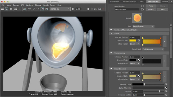
Figure 12.33 Render the molten metal in mental ray.
Emitting nParticles Using a Texture
The behavior of nParticles is often determined by their many dynamic properties. These properties control how the nParticles react to the settings in the Nucleus solver as well as fields, collision objects, and other nParticle systems. In the following section, you’ll get more practice working with these settings.
Surface Emission
In this exercise, you’ll use nParticles to create the effect of flames licking the base of a space capsule as it reenters the atmosphere. You’ll start by emitting nParticles from the base of the capsule and use a texture to randomize the generation of the nParticles on the surface.
- Open the
capsule_v01.mascene from thechapter12scenesdirectory at the book’s web page. You’ll see a simple polygon capsule model. The capsule is contained in a group named spaceCapsule. In the group, there is another surface named capsuleEmitter. This will serve as the surface emitter for the flames (see Figure 12.34). - Set a camera to the renderCam. Play the animation. The capsule has expressions that randomize the movement of the capsule to make it vibrate. The expressions are applied to the Translate channels of the group node. To see the expressions, do the following:
- Open the Expression Editor (Windows ➢ Animation Editors ➢ Expression Editor).
- Choose Select Filter ➢ By Expression Name.
-
Select expression1, expression2, or expression3.
You’ll see the expression in the box at the bottom of the editor (see Figure 12.35).
- In the viewport, choose to look through the renderCam. The camera has been set up so that the capsule looks as though it’s entering the atmosphere at an angle.
- In the Outliner, expand the spaceCapsule and choose the capsuleEmitter object.
- Switch to the FX menu set, and choose nParticles ➢ Create Options ➢ Point to set the nParticle style to Points.
- Select the capsuleEmitter, and choose nParticles ➢ Emit From Object ➢ Options.
- In the options, choose Edit ➢ Reset Settings to clear any settings that remain from previous Maya sessions.
- Set Emitter Name to flameGenerator. Set Emitter Type to Surface and Rate (Particles/Sec) to 150. Leave the rest of the settings at their defaults, and click the Apply button to create the emitter.
- Rewind and play the animation. The nParticles are born on the emitter and then start falling through the air. This is because the Nucleus solver has Gravity activated by default. For now this is fine; leave the settings on the Nucleus solver where they are.

Figure 12.34 The capsule group consists of two polygon meshes. The base of the capsule has been duplicated to serve as an emitter surface.

Figure 12.35 Create the vibration of the capsule using random function expressions applied to each of the translation channels of the capsule.
To randomize the generation of the nParticles, you can use a texture. To help visualize how the texture creates the particles, you can apply the texture to the surface emitter:
- Select the capsuleEmitter, and open the UV Editor (Windows ➢ UV Editor). You can see that the base already has UVs projected on the surface.
- Select the capsuleEmitter, right-click the surface in the viewport, and use the context menu to create a new Lambert texture for the capsuleEmitter surface. Name the shader flameGenShader.
- Open the Attribute Editor for flameGenShader, and click the checkered box to the right of the Color channel to create a new render node for color.
- In the Create Render Node window, click Ramp to create a ramp texture.
- In the Attribute Editor for the ramp (it should open automatically when you create the ramp), name the ramp flameRamp. Make sure that texture view is on in the viewport so that you can see the ramp on the capsuleEmitter surface (hot key = 6).
- Set the ramp’s type to Circular Ramp, and set Interpolation to None.
- Click the second color swatch, and use the Color Chooser to change it to white. Slide the white color swatch to about the halfway point on the ramp.
- Set Noise to 0.5 and Noise Freq to 0.3 to add some variation to the pattern (see Figure 12.36).
- In the Outliner, select the nParticle node and hide it (hot key = Ctrl+h) so that you can animate the ramp without having the nParticle simulation slow down the playback. Set the renderer to Legacy High Quality Viewport.
- Select the flameRamp node, and open it in the Attribute Editor. (Select the node by choosing it from the Textures area of the Hypershade.)
- Rewind the animation, and drag the white color marker on the ramp toward the left. Its Selected Position should be at 0.05.
- Right-click Selected Position, and choose Set Key (see Figure 12.37).
- Set the timeline to frame 100, move the white color marker all the way to the right of the ramp, and set another key for the Selected Position.
- Play the animation; you’ll see the dark areas on the ramp grow over the course of 100 frames.
- Open the Graph Editor (Windows ➢ Animation Editors ➢ Graph Editor). Click the Select button at the bottom of the ramp’s Attribute Editor to select the node; you’ll see the animation curve appear in the Graph Editor.
- Select the curve, switch to the Insert Keys tool, and add some keyframes to the curve.
- Use the Move tool to reposition the keys to create an erratic motion to the ramp’s animation (see Figure 12.38).
- In the Outliner, select the capsuleEmitter node and expand it.
- Select the flameGenerator emitter node, and open its Attribute Editor.
- Scroll to the bottom of the editor, and expand Texture Emission Attributes.
- Open the Hypershade to the Textures tab.
- MMB-drag flameRamp from the Textures area onto the color swatch for Texture Rate to connect the ramp to the emitter (see Figure 12.39).
- Select Enable Texture Rate and Emit From Dark.
- Increase Rate to 2400, unhide the nParticle1 node, and play the animation. You’ll see that the nParticles are now emitted from the dark part of the ramp.
- Select the capsuleEmitter node and hide it. Save the scene as
capsule_v02.ma.

Figure 12.36 Apply the ramp to the shader on the base capsuleEmitter object.

Figure 12.37 Position the white color marker at the bottom of the ramp and keyframe it.

Figure 12.38 Add keyframes to the ramp’s animation on the Graph Editor to make a more erratic motion.

Figure 12.39 Drag the ramp texture with the MMB from the Hypershade onto the Texture Rate color swatch to make a connection.
To see a version of the scene up to this point, open capsule_v02.ma from the chapter12scenes folder at the book’s web page.
Using Wind
The Nucleus solver contains settings to create wind and turbulence. You can use these settings with nParticles to create snow blowing in the air, bubbles rising in water, or flames flying from a careening spacecraft.
Now that you have the basic settings for the particle emission, the next task is to make the particles flow upward rather than fall. You can do this using either an air field or the Wind settings on the Nucleus solver. Using the Wind settings on the Nucleus solver applies wind to all nDynamic nodes (nCloth, nRigid, and nParticles) connected to the solver. In these steps, you’ll use the Nucleus solver. Fields will be discussed later in this chapter.
- Continue with the scene from the previous section, or open the
capsule_v02.mafile from thechapter12scenesdirectory. - Select the nParticle1 object in the Outliner. Rename it flames.
- Open the Attribute Editor, and choose the nucleus1 tab.
- Set Gravity to 0, and play the animation. The particles emerge from the base of the capsule and stop after a short distance. This is because by default the nParticles have a Drag value of 0.01 set in their Dynamic Properties settings.
- Switch to the flamesShape tab, expand the Dynamic Properties rollout panel, and set Drag to 0. Play the animation, and the nParticles emerge and continue to travel at a steady rate.
- Switch back to the nucleus1 tab:
- Set the Wind Direction fields to 0, 1, 0 so that the wind is blowing straight up along the y-axis.
- Set Wind Speed to 5 (see Figure 12.40).
-
Play the animation.
There’s no change; the nParticles don’t seem affected by the wind.
For the Wind settings in the Nucleus solver to work, the nParticle needs to have a Drag value, even a small one. This is why all of the nParticle styles except Water have drag applied by default. If you create a Water-style particle and add a Wind setting, it won’t affect the water until you set the Drag field above 0. Think of drag as a friction setting for the wind. In fact, the higher the Drag setting, the more the wind can grab the particle and push it along, so it actually has a stronger pull on the nParticle.
- Switch to the tab for the flamesShape, set the Drag value to 0.01, and play the animation. The particles now emerge and then move upward through the capsule.
-
Switch to the nucleus1 tab; set Air Density to 5 and Wind Speed to 25. The Air Density setting also controls, among other things, how much influence the wind has on the particles.
A very high air density acts like a liquid, and a high wind speed acts like a current in the water. It depends on what you’re trying to achieve in your particular effect, but you can use drag or air density or a combination to set how much influence the Wind settings have on the nParticle. Another attribute to consider is the particle’s mass. Since these are flames, presumably the mass will be very low.
- Set Air Density to 1. Rewind and play the animation. The particles start out slowly but gain speed as the wind pushes them along.
- Set the Mass attribute in the Dynamic Properties section of the flamesShape tab to 0.01. The particles are again moving quickly through the capsule (see Figure 12.41).
- Switch to the nucleus1 tab, and set Wind Noise to 10. Because the particles are moving fast, Wind Noise needs to be set to a high value before there’s any noticeable difference in the movement. Wind noise adds turbulence to the movement of the particles as they are pushed by the wind.
- To make the nParticles collide with the capsule, select the capsule node and choose nCloth ➢ Create Passive Collider. The nParticles now move around the capsule.
- Select the nRigid1 node in the Outliner, and name it flameCollide.
- Under the Collisions section, expand the Wind Field Generation settings in the flameCollideShape node. Set Air Push Distance to 0.5 and Air Push Vorticity to 1.5 (see Figure 12.42).
- Save the scene as
capsule_v03.ma.

Figure 12.40 The settings for the wind on the nucleus1 tab

Figure 12.41 Set the Mass and Drag attributes to a low value, enabling the nParticle flames to be pushed by the wind on the Nucleus solver.

Figure 12.42 The Wind Field Generation settings on the flameCollideShape node
To see a version of the scene up to this point, open capsule_v03.ma from the chapter12scenes folder at the book’s web page.
A passive object can generate wind as it moves through particles or nCloth objects to create the effect of air displacement. In this case, the capsule is just bouncing around, so the Air Push Distance setting helps jostle the particles once they have been created. If you were creating the look of a submarine moving through murky waters with particulate matter, the Air Push Distance setting could help create the look of the particles being pushed away by the submarine, and the Air Push Vorticity setting could create a swirling motion in the particles that have been pushed aside. In the case of the capsule animation, it adds more turbulence to the nParticle flames.
The Wind Shadow Distance and Diffusion settings block the effect of the Nucleus solver’s Wind setting on nParticles or nCloth objects on the side of the passive object opposite the direction of the wind. The Wind Shadow Diffusion attribute sets the degree to which the wind curls around the passive object.
Air Push Distance is more processor-intensive than Wind Shadow Distance, and the Maya documentation recommends that you not combine Air Push Distance and Wind Shadow Distance.
nParticles have these settings as well. You can make an nParticle system influence an nCloth object using the Air Push Distance setting.
Shading nParticles and Using Hardware Rendering to Create Flame Effects
Once you have created your nParticle simulation, you’ll have to decide how to render the nParticles in order to best achieve the effect you want. The first decision that you’ll have to make is how to shade the nParticles—how they will be colored and what rendering style will best suit your needs. Maya makes this process fairly easy because there are several rendering styles to choose from, including Points, MultiPoint, Blobby Surface, Streak, MultiStreak, and Cloud. Any one of these styles will change the appearance of the individual nParticles and thus influence the way the nParticle effect looks in the final rendered image.
To make coloring the nParticles easy, Maya provides you with a number of colored ramps that control the nParticles’ color, opacity, and incandescence over time. You can choose different attributes, such as Age, Acceleration, Randomized ID, and so on, to control the way the color ramps are applied to the nParticles. You can find all of these attributes in the Shading section of the nParticle’s Attribute Editor.
Most of the time, you’ll want to render nParticles as a separate pass from the rest of the scene and then composite the rendered nParticle image sequence together with the rest of the rendered scene in your compositing program. This is so that you can easily isolate the nParticles and apply effects such as blurring, glows, and color correction separately from the other elements of the scene. You have a choice as to how you can render the nParticles. This can be done using mental ray, Maya Software, Maya Hardware, or the Hardware Render Buffer. This section demonstrates how to render using the Hardware Render Buffer. Later in the chapter you’ll learn how to render nParticles using mental ray.
Shading nParticles to Simulate Flames
Color and opacity attributes can be easily edited using the ramps in the nParticle’s Attribute Editor. In these steps, you’ll use these ramps to make the nParticles look more like flames:
- Continue with the same scene from the previous section, or open
capsule_v03.mafrom thechapter12scenesfolder at the book’s web page. -
Select the flames nParticle node in the Outliner, and open the Attribute Editor to the flamesShape node. Expand the Lifespan rollout panel, and set Lifespan Mode to Random Range. Set Lifespan to 3 and Lifespan Random to 3.
This setting makes the average life span for each nParticle 3 seconds, with a variation of half the Lifespan Random setting in either direction. In this case, the nParticles will live anywhere between 0.5 and 4.5 seconds.
- Scroll down to the Shading rollout panel, and expand it; set Particle Render Type to MultiStreak. This makes each nParticle a group of streaks and activates attributes specific to this render type.
- Set Multi Count to 5, Multi Radius to 0.8, and Tail Size to 0.5 (see Figure 12.43).
-
In the Opacity Scale section, set Opacity Scale Input to Age. Click the right side of the Opacity Scale ramp curve to add an edit point. Drag this point down. This creates a ramp where the nParticle fades out over the course of its life (see Figure 12.44).
If you’ve used standard particles in older versions of Maya, you know that you normally have to create a per-particle Opacity attribute and connect it to a ramp. If you scroll down to the Per Particle Array Attributes section, you’ll see that Maya has automatically added the Opacity attribute and connected it to the ramp curve.
- Set Input Max to 1.5. This sets the maximum range along the x-axis of the Opacity Scale ramp. Since Opacity Scale Input is set to Age, this means that each nParticle takes 1.5 seconds to become transparent, so the nParticles are visible for a longer period of time.
- To randomize the opacity scale for the opacity, set Opacity Scale Randomize to 0.5.
- Expand the Color rollout panel. Set Color Input to Age. Click the ramp just to the right of the color marker to add a new color to the ramp. Click the color swatch, and change the color to yellow.
- Add a third color marker to the right end of the ramp, and set its color to orange.
- Set Input Max to 2 and Color Randomize to 0.8, as in Figure 12.44.
- In the Shading section, enable Color Accum. This creates an additive color effect, where denser areas of overlapping particles appear brighter.
- Save the scene as
capsule_v04.ma.

Figure 12.43 Change Particle Render Type to MultiStreak to better simulate flames.

Figure 12.44 The opacity and color ramps in the nParticle’s attribute replace the need to connect ramps manually.
To see a version of the scene up to this point, open capsule_v04.ma from the chapter12scenes folder at the book’s web page.
Creating an nCache
Before rendering, it’s always a good idea to create a cache to ensure that the scene renders correctly.
- Continue with the scene from the previous section, or open the
capsule_v04.mafile from thechapter12scenesfolder at the book’s web page. - Set the timeline to 200 frames.
- In the Outliner, expand the capsuleEmitter group and select the flameGenerator emitter. Increase Rate (Particle/Sec) to 25000. This will create a much more believable flame effect.
-
Select the flames node in the Outliner. In the FX menu set, choose nCache ➢ Create New Cache ➢ nObject ➢ Options. In the options, you can choose a name for the cache or use the default, which is the name of the selected node (flamesShape in this example). You can also specify the directory for the cache, which is usually the project’s
datadirectory. Leave File Distribution set to One File Per Frame and Cache Time Range to Time Slider. Click Create to make the cache (see Figure 12.45).The scene will play through, and the cache file will be written to disk. It will take a fair amount of time to create the cache—anywhere from 5 to 10 minutes, depending on the speed of your machine.
- Open the Attribute Editor for the flamesShape tab, and uncheck the Enable button so that the nParticle is disabled. This prevents Maya from calculating the nParticle dynamics while using an nCache.
- Play the animation, and you’ll see the nParticles play back even though they have been disabled.
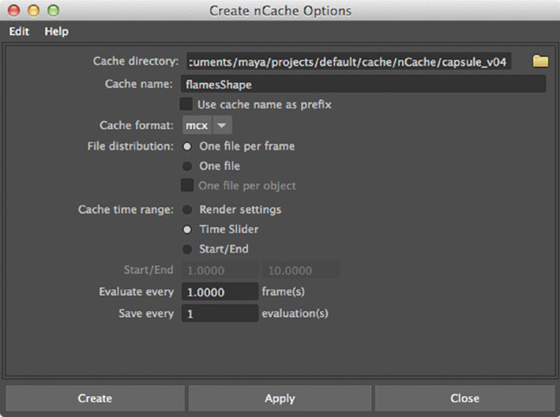
Figure 12.45 The options for creating an nCache
The playback is much faster now since the dynamics do not have to be calculated. If you make any changes to the dynamics of the nParticles, you’ll have to delete or disable the existing cache before you’ll see the changes take effect.
By default, only the Position and Velocity attributes of the nParticle are stored when you create an nCache. If you have a more complex simulation in which other attributes change over time (such as mass, stickiness, rotation, and so on), then open the Caching rollout panel in the nParticle’s Attribute Editor, set Cacheable Attributes to All, and create a new nCache (see Figure 12.46). It is a fairly common mistake to forget to do this, and if you do not cache all of the attributes, you’ll notice that the nParticles do not behave as expected when you play back from the nCache or when you render the animation. The nCache file will be much larger when you change the Cacheable Attributes setting.

Figure 12.46 Set Cacheable Attributes to All when you want to cache attributes other than just Position and Velocity.
You can use the options in the nCache menu to attach an existing cache file to an nParticle or to delete, append, merge, or replace caches.
Using the Hardware Render Buffer
One of the fastest and easiest ways to render flames in Maya is to use the Hardware Render Buffer. The results may need a little extra tweaking in a compositing program, but overall it does a decent job of rendering convincing flames. The performance of the Hardware Render Buffer depends on the type of graphics card installed in your machine. If you’re using an Autodesk-approved graphics card, you should be in good shape.
The Blobby Surface, Cloud, and Tube nParticle render styles can be rendered only using software (Maya Software or mental ray). All nParticle types can be rendered in mental ray, although the results may be different than those rendered using the Hardware Render Buffer or Maya Hardware. The following steps explain how you use the Hardware Render Buffer to render particles.
- Continue from the previous section. To render using the Hardware Render Buffer, choose Windows ➢ Rendering Editors ➢ Hardware Render Buffer. A new window opens showing a wireframe display of the scene. Use the Cameras menu in the buffer to switch to the renderCam camera.
-
To set the render attributes in the Hardware Render Buffer, choose Render ➢ Attributes. The settings for the buffer appear in the Attribute Editor.
The render buffer renders each frame of the sequence and then takes a screenshot of the screen. It’s important to deactivate screen savers and keep other interface or application windows from overlapping the render buffer.
- For Filename, type capsuleFlameRender, and for Extension, enter name.0001.ext.
-
Set Start Frame to 1 and End Frame to 200. Keep By Frame set to 1.
Keep Image Format set to Maya IFF. This file format is compatible with compositing programs such as Adobe After Effects.
- To change the resolution, you can manually replace the numbers in the Resolution field or click the Select button to choose a preset. Click this button, and choose the 640 × 480 preset.
- In the viewport window, you may want to turn off the display of the resolution or film gate. The view in the Hardware Render Buffer updates automatically.
- Under Render Modes, select Full Image Resolution and Geometry Mask. Geometry Mask renders all of the geometry as a solid black mask so that only the nParticles will render. You can composite the rendered particles over a separate pass of the software-rendered version of the geometry.
- To create the soft look of the frames, expand the Multi-Pass Render Options rollout panel. Select Multi Pass Rendering, and set Render Passes to 36. This means that the buffer will take 36 snapshots of the frame and slightly jitter the position of the nParticles in each pass. The passes will then be blended together to create the look of the flame. For flame effects, this actually works better than the buffer’s Motion Blur option. Leave Motion Blur at 0 (see Figure 12.47).
- Rewind and play the animation to about frame 45.
- In the Hardware Render Buffer, click the clapboard icon to see a preview of how the render will look (see Figure 12.48).
- If you’re happy with the look, choose Render ➢ Render Sequence to render the 200-frame sequence. It should take 5 to 10 minutes depending on your machine. You’ll see the buffer render each frame.
- When the sequence is finished, choose Flipbooks ➢ capsuleFlameRender1-200 to see the sequence play in FCheck.
- Save the scene as
capsule_v05.ma.

Figure 12.47 The settings for the Hardware Render Buffer

Figure 12.48 When Geometry Mask is enabled, the Hardware Render Buffer renders only the nParticles.
To see a version of the scene up to this point, open the capsule_v05.ma scene from the chapter12scenes directory at the book’s web page.
To finalize the look of flames, you can apply additional effects such as glow and blur in your compositing program. Take a look at the capsuleReentry movie in the chapter12 folder at the book’s web page to see a finished movie made using the techniques described in this section.
Controlling nParticles with Fields
Fields are used most often to control the behavior of nParticles. There are three ways to generate a field for an nParticles system. First, you can connect one or more of the many fields listed in the Fields menu. These include Air, Drag, Gravity, Newton, Radial, Turbulence, Uniform, Vortex, and Volume Axis Curve. Second, you can use the fields built into the Nucleus solver—these are the Gravity and Wind forces that are applied to all nDynamic systems connected to the solver. Finally, you can use the Force field and the Air Push fields that are built into nDynamic objects. In this section, you’ll experiment with using all of these types of fields to control nParticles.
Using Multiple Emitters
When you create the emitter, an nParticle object is added and connected to the emitter. An nParticle can be connected to more than one emitter, as you’ll see in this exercise:
- Open the
generator_v01.mascene in thechapter12scenesfolder at the book’s web page. You’ll see a device built out of polygons. This will act as your experimental lab as you learn how to control nParticles with fields. - Switch to the FX menu set, and choose nParticles ➢ Create Options ➢ Cloud to set the nParticle style to Cloud.
- Choose nParticles ➢ Create Emitter ➢ Options.
- In the options, type energyGenerator in the Emitter Name field. Leave Solver set to Create New Solver. Set Emitter Type to Volume and Rate (Particles/Sec) to 200.
- In the Volume Emitter Attributes rollout panel, set Volume Shape to Sphere. You can leave the rest of the settings at the defaults. Click Create to make the emitter (see Figure 12.49).
- Select the energyGenerator1 emitter in the Outliner. Use the Move tool (hot key = w) to position the emitter around one of the balls at the end of the generators in the glass chamber. You may want to scale it up to about 1.25 (see Figure 12.50).
-
Set the timeline to 800, and play the animation. The nParticles are born and fly out of the emitter.
Notice that the nParticles do not fall even though Gravity is enabled in the Nucleus solver and the nParticle has a mass of 1. This is because in the Dynamic properties for the Cloud style of nParticle, the Ignore Solver Gravity check box is selected.
-
Select the energyGenerator1 emitter, and duplicate it (hot key = Ctrl/Cmd+d). Use the Move tool to position this second emitter over the ball on the opposite generator.
If you play the animation, the second emitter creates no nParticles. This is because duplicating the emitter did not create a second nParticle object, but that’s okay; you’re going to connect the same nParticle object to both emitters.
- Select nParticle1 in the Outliner, and rename it energy.
- Select energy, and choose Windows ➢ Relationship Editors ➢ Dynamic Relationships. A window opens showing the objects in the scene; energy is selected on the left side.
- On the right side, click the Emitters radio button to switch to a list of the emitters in the scene. energyGenerator1 is highlighted, indicating that the energy nParticle is connected to it.
- Select energyGenerator2 so that both emitters are highlighted (see Figure 12.51).
- Close the Dynamic Relationships Editor, and rewind and play the animation. You’ll see both emitters now generate nParticles—the same nParticle object.
- Select the energy object, and open the Attribute Editor. Switch to the Nucleus tab, and set Gravity to 1.
- In the energyShape tab, expand the Dynamic Properties rollout panel, and deselect Ignore Solver Gravity so that the energy nParticles slowly fall after they are emitted from the two generator poles (see Figure 12.52).

Figure 12.49 The settings for the volume emitter

Figure 12.50 Place the volume emitter over one of the balls inside the generator device.

Figure 12.51 Use the Dynamic Relationships Editor to connect the energy nParticle to both emitters.

Figure 12.52 The energy nParticles are emitted from both emitters. Gravity is set to a low value, causing the nParticles to fall slowly.
Volume Axis Curve
Volume Axis Curve is a versatile dynamic field that can be controlled using a NURBS curve. You can use this field with any of the dynamic systems in Maya. In this section, you’ll perform some tricks using the field inside a model of an experimental vacuum chamber.
- Select the energy nParticle node in the Outliner. In the Attribute Editor, open the Lifespan rollout panel and set the Lifespan mode to Random Range.
- Set Lifespan to 6 and Lifespan Random to 4. The nParticles will now live between 4 and 8 seconds each.
- With the energy nParticle selected, choose Fields/Solvers ➢ Volume Curve. Creating the field with the nParticle selected ensures that the field is automatically connected.
- Select curve1 in the Outliner, and use the Move tool to position it between the generators. The field consists of a curve surrounded by a tubular field.
- Use the Show menu to disable the display of polygons so that the glass case is not in the way.
- Select curve1 in the Outliner, and right-click the curve; choose CVs to edit the curve’s control vertices.
- Use the Move tool to position the CVs at the end of the curve inside each generator ball, and then add some bends to the curve (see Figure 12.53).
- Rewind and play the animation. A few of the nParticles will be pushed along the curve. So far, it’s not very exciting.
- Select the volumeAxisField1 node in the Outliner, and open its Attribute Editor. Use the following settings:
- The default Magnitude and Attenuation settings (5 and 0) are fine for the moment.
- In the Distance rollout panel, leave Use Max Distance deselected.
- In the Volume Control Attributes rollout panel, set Section Radius to 3.
- Set Trap Inside to 0.8. This keeps most of the nParticles inside the area defined by the volume radius (the Trap Inside attribute is available for other types of fields such as the Radial field).
- Leave Trap Radius set to 2. This defines the radius around the field within which the nParticles are trapped.
- Edit the Axial Magnitude ramp so that each end is at about 0.5 and the middle is at 1, as shown in Figure 12.54. Set the interpolation of each point to Spline. This means that the area at the center of the curve has a stronger influence on the nParticles than the areas at either end of the curve.
- Edit the Curve Radius ramp: add some points to the curve, and drag them up and down in a random jagged pattern. You’ll see the display of the field update; this creates an interesting shape for the curve.
- In the Volume Speed Attributes rollout panel, set Away From Axis and Along Axis to 0, and set Around Axis to 4. This means that the nParticles are pushed in a circular motion around the curve rather than along or away from it. If you zoom into the field, you’ll see an arrow icon at the end of the field indicating its direction. Positive numbers make the field go clockwise; negative numbers make it go counterclockwise.
- Set Turbulence to 3, and leave Turbulence Speed at 0.2. This adds noise to the field, causing some nParticles to fly off.
-
Play the animation. You’ll see the nParticles move around within the field. Faster-moving particles fly out of the field.
This effect is interesting, but it can be improved to create a more dynamic look.
- In the Attribute Editor for the Volume Axis Curve field, remove the edit points from the Curve Radius ramp.
- Edit the curve so that it has three points. The points at either end should have a value of 1; the point at the center should have a value of 0.1.
- Select the edit point at the center and, in the Selected Position field, type
=0.5+(0.5*(noise(time*4)));. This is similar to the expression that was applied to the ramp in the “Surface Emission” section earlier in this chapter. In this case, it moves the center point back and forth along the curve, creating a moving shape for the field (see Figure 12.55). - Save the scene as
generator_v02.ma.

Figure 12.53 Position the CVs of the Volume Axis curve to add bends to the curve. The field surrounds the curve, forming a tube.

Figure 12.54 The settings for the Volume Axis Curve field

Figure 12.55 Create an expression to control the Selected Position attribute of the Curve Radius ramp’s center point. The numeric field is not large enough to display the entire expression.
To see a version of the scene up to this point, open the generator_v02.ma scene from the chapter12scenes folder at the book’s web page. This version uses a Dynamic Hair curve to control the field. To learn how to use this technique, refer to the sidebar “Using a Dynamic Hair Curve with a Volume Axis Curve.”
Working with Force Fields
nParticles, nCloth, and passive collision objects (also known as nRigids) can all emit force fields that affect themselves and other nDynamic systems attached to the same Nucleus node. In this example, the surface of the glass that contains the particle emitters will create a field that controls the nParticle’s behavior:
- Continue with the scene from the previous section, or open the
generator_v02.mascene from thechapter12scenesfolder at the book’s web page. - Expand the housing group in the Outliner. Select the dome object, and choose nCloth ➢ Create Passive Collider.
- In the Outliner, rename the nRigid1 node to domeCollider.
- To keep the particles from escaping the chamber, you’ll also need to convert the seal and base objects to passive collision objects:
- Select the seal object, and choose nCloth ➢ Create Passive Collider.
- Name the new nRigid1 node sealCollide.
- Do the same for the base, and name it baseCollide.
- Play the animation. Because some of the nParticles are thrown from the Volume Axis Curve field, they are now contained within the glass chamber (see Figure 12.56).
- Open the settings for the energyShape node in the Attribute Editor. In the Particle Size rollout panel, make sure that Radius Scale Input is set to Age.
- Edit the Radius Scale ramp so that it slopes up from 0 on the left to 1 in the middle and back down to 0 on the left.
- Set Interpolation to Spline for all points along the curve.
- Set Input Max to 3 and Radius Scale Randomize to 0.5 (see Figure 12.57).
- Select the domeCollider node, and open the Attribute Editor to the domeColliderShape tab.
-
Expand the Force Field Generation settings, and set Force Field to Single Sided. This generates a force field based on the positive normal direction of the collision surface.
Along Normal generates the field along the surface normals of the collision object. In this case, the difference between Along Normal and Single Sided is not noticeable. Double Sided generates the field based on both sides of the collision surface.
- The normals for the dome shape are actually pointing outward. You can see this if you choose Display ➢ Polygons ➢ Face Normals. To reverse the surface, switch to the Modeling menu set, and choose Mesh Display ➢ Reverse (see Figure 12.58).
- Back in the Force Field Generation settings for the domeColliderShape node, set Field Magnitude to 100 and Field Distance to 4, and play the animation. The particles are repelled from the sides of the dome when they are within 4 field units of the collision surface. A lower field magnitude will repel the particles with a weaker force, allowing them to collide with the dome before being pushed back to the center. If you set Magnitude to 1000, the nParticles never reach the collision surface.
-
Set Field Magnitude to −100. The nParticles are now pulled to the sides of the dome when they are within 4 field units of the collision surface, much like a magnet. Setting a value of −1000 causes them to stick to the sides.
The Field Scale ramp editor controls the strength of the field within the distance set by the Field Distance value. The right side of the ramp is the leading edge of the field—in this case, 4 field units in from the surface of the dome. The left side represents the scale of the force field on the actual collision surface.
You can create some interesting effects by editing this curve. If Field Magnitude is at a value of −100 and you reverse the curve, the nParticles are sucked to the dome quickly when they are within 4 units of the surface. However, they do not stick very strongly to the side, so they bounce around a little within the 4-unit area. Experiment with creating different shapes for the curve, and see how the curve affects the behavior of the nParticles. By adding variation to the center of the curve, you get more of a wobble as the nParticle is attracted to the surface.
- Save the scene as
generator_v03.ma.

Figure 12.56 Parts of the generator device are converted to collision objects, trapping the nParticles inside.

Figure 12.57 Edit the Radius Scale settings to create a more randomized radius for the nParticles.

Figure 12.58 Reverse the normals for the dome surface so that they point inward.
To see a version of the scene to this point, open the generator_v03.ma scene from the chapter12scenes folder at the book’s web page.
Painting Field Maps
The strength of the force field can be controlled by a texture. The texture itself can be painted onto the collision surface.
- Continue with the scene from the previous section, or open the
generator_v03.mascene from thechapter12scenesfolder at the book’s web page. - In the Attribute Editor for domeColliderShape, set the Field Scale ramp so that it’s a straight line across the top of the curve editor. Set Field Magnitude to 1.
- Select the dome object under the Housing group, and choose nCloth ➢ Paint Texture Properties ➢ Field Magnitude. The dome turns white, and the Artisan Brush tool is activated. If the dome turns black, open the Flood controls in the Artisan Tool options and click the Flood Paint button to fill the surface with a value of 1 for the Field Strength attribute.
- In the tool settings for the Artisan Brush, Color should be set to black and Paint Operations should be set to Paint.
- Use the brush to paint a pattern on the surface of the dome. Make large, solid lines on the surface so that the end result is clear. Avoid blurring the edges (see Figure 12.59).
- When you’ve finished, click the Select tool in the toolbox to close the Artisan Brush options.
- Open the Hypershade. On the Textures tab, you’ll see the texture map that you just created. You can also use file textures or even animated sequences for the map source.
- Select the dome in the scene. In the Node Editor area of the Hypershade, right-click and choose Graph Materials On Viewport Selection. Select the domeShader in the Node Editor.
-
MMB-drag the file1 texture from the Palette area of the Hypershade onto the Color And Transparency channel in the Property Editor. Connecting the texture to the color does not affect how the field works, but it will help you visualize how the map works (see Figure 12.60).
If you play the animation, you won’t see much of a result. The reason is that the values of the map are too weak and the movement of the nParticles is too fast to be affected by the field.
- In the Hypershade, choose the Input and Output Connections icon from within the Node Editor panel. Select the file1 texture to expose its attributes in the Property Editor. The outAlpha of the texture is connected to the field magnitude of the collision surface. You can see this when you graph the network in the Node Editor panel.
- To increase the strength of the map, expand the Color Balance section. Set Alpha Gain to 1000 and Alpha Offset to −500. Chapter 16, “Scene Management and Virtual Filmmaking,” has a detailed explanation of how the Alpha Gain and Alpha Offset attributes work. Essentially, this means that the light areas of the texture cause the force field magnitude to be at a value of 500, and the dark areas cause it to be at −500.
-
Play the animation. You’ll see that most of the nParticles stay in the center of the dome, but occasionally one or two nParticles will fly out and stick to the side. They stick to the areas where the texture is dark (see Figure 12.61).
Vertex maps assign values to the vertices of the surface using the colors painted by the brush; texture maps use a file texture. One may work better than the other depending on the situation. You can paint vertex maps by choosing nCloth ➢ Paint Vertex Properties. In the Map properties, set Map Type to Vertex or Texture, depending on which one you are using.
When using a texture or vertex map for the force field, the Force Field Magnitude setting acts as a multiplier for the strength of the map.
- Back in the domeCollider node, set Field Magnitude to 10 and play the animation. You’ll see more nParticles stick to the surface where the texture has been painted. To smooth their motion, you can adjust the Field Scale ramp.
- Save the scene as
generator_v04.ma.

Figure 12.59 Use the Artisan Brush tool to paint a pattern for the field magnitude on the collision surface.

Figure 12.60 Connect the newly painted texture to the color of the dome shader.

Figure 12.61 The painted force field texture causes most of the nParticles to remain hovering around the center, but a few manage to stick to the dark areas.
To see a version of the scene up to this point, open generator_v04.ma from the chapter12scenes folder at the book’s web page.
Using Dynamic Fields
The traditional set of dynamic fields is found in the Fields/Solvers menu. They have been included as part of Maya since version 1.
Fields such as Air and Gravity are similar to the wind and gravity forces that are part of the Nucleus system. But that is not to say you that can’t use them in combination with the Nucleus forces to create a specific effect.
Drag is similar to the Drag attribute of nParticles; it applies a force that, in some cases, slows an nParticle down; in other cases, it actually pulls the nParticle in a direction determined by the force. You can use the Inherit Transform slider on the Drag field to create wavelike effects in a cloud of particles, similar to the wind field generation on nDynamic objects.
Radial fields are similar to force fields emitted by nRigids and nParticles; they push or pull particles, depending on their Magnitude settings.
A Uniform force is similar to Gravity because it pushes a particle in a particular direction. The Volume Axis field is similar to the Volume Curve used earlier in the chapter. It has a built-in turbulence and affects particles within a given volume shape (by default).
The Turbulence field creates a noise pattern, and the Vortex field creates a swirling motion. Newton fields create a Newtonian attraction to dynamic objects.
- Open the
generator_v04.mascene from thechapter12scenesfolder at the book’s web page. - Select the energy nParticle group, and choose Fields/Solvers ➢ Turbulence to connect a Turbulence field to the nParticle.
- In the Attribute Editor for the Turbulence field, set Magnitude to 100, Attenuation to 0, and Frequency to 0.5.
- In the Dynamic Properties section of the nParticle’s Attribute Editor, set Drag to 0.1. This can help tone down the movement of the nParticles if they get a little too crazy. An alternative technique is to lower the conserve a little.
- To see the particles behave properly, you’ll probably want to create a playblast. Set the timeline to 300, and choose Windows ➢ Playblast. A flip book will be created and played in FCheck.
- Save the scene as
generator_v05.ma.
To see a version of the scene up to this point, open generator_v05.ma from the chapter12scenes folder at the book’s web page.
Rendering Particles with mental ray
All particle types can be rendered using mental ray software rendering, and particles will appear in reflections and refractions. In this section, you’ll see how easy it is to render different nParticle types using mental ray.
In this exercise, you’ll render the nParticles created in the generator scene:
- Open the
generator_v05.mascene from thechapter12scenesfolder at the book’s web page or continue from the previous section. - Select the energy nParticle node in the Outliner, and open its Attribute Editor to the energyShape tab.
- Expand the Shading attributes in the bottom of the editor. Set Opacity to 0.8.
- Set Color Input to Age. Make the left side of the ramp bright green and the right side a slightly dimmer green.
- Set Incandescence Input to Age. Edit the ramp so that the far-left side is white, followed closely by bright green. Make the center a dimmer green and the right side completely black (see Figure 12.62).
- Select each of the emitter nodes, and raise the Rate value to 1000.
- Select the domeShader node in the Hypershade, and break the connection between the color and the file texture. (Don’t delete the file texture—it still controls the force field magnitude.)
- Set the color of the domeShader node to a dark gray.
- Play the animation for about 80 frames.
- Open the render settings, and set the renderer to mental ray.
- From the Presets menu, choose Load Preset ➢ Production.
- Select the energy nParticle and, in the Render Stats section of the energyShape tab, select the boxes for Visible in Reflections and Refractions.
- Create a test render of the scene. You can see in the glass of the chamber and the metal base that the nParticles are reflected.
- Open the Hypershade, and select the metal shader. Increase Reflectivity in the Attribute Editor to 0.8. The nParticles are more visible in the reflection on the base.
- Select the domeShader node, and in its Attribute Editor under Raytrace Options, select Refractions and set Refractive Index to 1.2.
- Under the Specular Shading rollout panel, increase Reflectivity to 0.8.
-
Create another test render. You can see the effect refraction has on the nParticles. Figure 12.63 shows both reflections and refractions.
You can render the Point, MultiPoint, Streak, and MultiStreak render types using mental ray. They will appear in reflections and refractions as well; however, you’ll notice that in the Render Stats section for these nParticle types, the options for Reflections and Refractions are unavailable.
-
In the Hypershade, select the npCloudVolume shader. This shader is created with the nParticle. Graph the network in the Hypershade Node Editor panel (see Figure 12.64).
You can see that a particleSamplerInfo node is automatically connected to the volume shader. This node transfers the settings that you create in the nParticle’s Attribute Editor for color, opacity, and transparency to the shader. An npCloudBlinn shader is also created. This shader is applied when you switch Particle Type to Points. You can further refine the look of the nParticles by adjusting the settings in the npCloudVolume shader’s Attribute Editor.
You can add a shader glow to the particles by increasing Glow Intensity in the npCloudVolume shader; however, the glow does not appear behind refractive surfaces with standard Maya shaders.
- When you are happy with the look of the render, you can create an nCache for the energy nParticle and render the sequence using mental ray.
- Save the scene as
generator_v06.ma.

Figure 12.62 The shading attributes for the energy nParticle

Figure 12.63 The nParticles are visible in reflections and refractions on the surfaces.

Figure 12.64 Shaders are automatically created for the nParticles. The particleSamplerInfo node connects the attributes of the nParticle to the shader.
To see a finished version of the scene, open the generator_v06.ma file from the chapter12scenes directory.
The Bottom Line
Create nParticles. nParticles can be added to a scene in a number of ways. They can be drawn using the nParticle tool or spawned from an emitter, or they can fill an object.
Master It Create a spiral shape using nParticles.
Make nParticles collide. nParticles can collide with themselves, other nParticles, and polygon surfaces.
Master It Make nParticles pop out of the top of an animated volume.
Create liquid simulations. Enabling Liquid Simulations changes the behavior of nParticles so that they act like water or other fluids.
Master It Create a flowing stream of nParticles that ends in a waterfall.
Emit nParticles from a texture. The emission rate of an nParticle can be controlled using a texture.
Master It Create your own name in nParticles.
Move nParticles with Nucleus wind. The wind force on the Nucleus node can be used to push nParticles.
Master It Blow nParticles off a surface using wind.
Use force fields. NParticles and collision objects can emit force fields, creating interesting types of behavior in your scenes.
Master It Add a second nParticle object emitted from the base of the generator. Enable its force field so that it attracts some of the original energy nParticle.